
Working with large data
Last updated on 2026-08-05 | Edit this page
Overview
Questions
- How do we work with single-cell datasets that are too large to fit in memory?
- How do we speed up single-cell analysis workflows for large datasets?
- How do we convert between popular single-cell data formats?
Objectives
- Work with out-of-memory data representations such as HDF5.
- Speed up single-cell analysis with parallel computation.
- Invoke fast approximations for essential analysis steps.
- Convert
SingleCellExperimentobjects toSeuratObjects andAnnDataobjects.
Motivation
Advances in scRNA-seq technologies have increased the number of cells that can be assayed in routine experiments. Public databases such as GEO are continually expanding with more scRNA-seq studies, while large-scale projects such as the Human Cell Atlas are expected to generate data for billions of cells. For effective data analysis, the computational methods need to scale with the increasing size of scRNA-seq data sets. This section discusses how we can use various aspects of the Bioconductor ecosystem to tune our analysis pipelines for greater speed and efficiency.
Out of memory representations
The count matrix is the central structure around which our analyses
are based. In most of the previous chapters, this has been held fully in
memory as a dense matrix or as a sparse
dgCMatrix. Howevever, in-memory representations may not be
feasible for very large data sets, especially on machines with limited
memory. For example, the 1.3 million brain cell data set from 10X
Genomics (Zheng et al.,
2017) would require over 100 GB of RAM to hold as a
matrix and around 30 GB as a dgCMatrix. This
makes it challenging to explore the data on anything less than a HPC
system.
The obvious solution is to use a file-backed matrix representation where the data are held on disk and subsets are retrieved into memory as requested. While a number of implementations of file-backed matrices are available (e.g., bigmemory, matter), we will be using the implementation from the HDF5Array package. This uses the popular HDF5 format as the underlying data store, which provides a measure of standardization and portability across systems. We demonstrate with a subset of 20,000 cells from the 1.3 million brain cell data set, as provided by the TENxBrainData package.
R
library(TENxBrainData)

sce.brain <- TENxBrainData20k()

sce.brain
OUTPUT
class: SingleCellExperiment
dim: 27998 20000
metadata(0):
assays(1): counts
rownames: NULL
rowData names(2): Ensembl Symbol
colnames: NULL
colData names(4): Barcode Sequence Library Mouse
reducedDimNames(0):
mainExpName: NULL
altExpNames(0):
Examination of the SingleCellExperiment object indicates
that the count matrix is a HDF5Matrix. From a comparison of
the memory usage, it is clear that this matrix object is simply a stub
that points to the much larger HDF5 file that actually contains the
data. This avoids the need for large RAM availability during
analyses.
R
counts(sce.brain)
OUTPUT
<27998 x 20000> HDF5Matrix object of type "integer":
             [,1]     [,2]     [,3]     [,4] ... [,19997] [,19998] [,19999]
    [1,]        0        0        0        0   .        0        0        0
    [2,]        0        0        0        0   .        0        0        0
    [3,]        0        0        0        0   .        0        0        0
    [4,]        0        0        0        0   .        0        0        0
    [5,]        0        0        0        0   .        0        0        0
     ...        .        .        .        .   .        .        .        .
[27994,]        0        0        0        0   .        0        0        0
[27995,]        0        0        0        1   .        0        2        0
[27996,]        0        0        0        0   .        0        1        0
[27997,]        0        0        0        0   .        0        0        0
[27998,]        0        0        0        0   .        0        0        0
         [,20000]
    [1,]        0
    [2,]        0
    [3,]        0
    [4,]        0
    [5,]        0
     ...        .
[27994,]        0
[27995,]        0
[27996,]        0
[27997,]        0
[27998,]        0
R
object.size(counts(sce.brain))
OUTPUT
2496 bytesR
file.size(path(counts(sce.brain)))
OUTPUT
[1] 76264332Manipulation of the count matrix will generally result in the
creation of a DelayedArray object from the DelayedArray
package. This remembers the operations to be applied to the counts and
stores them in the object, to be executed when the modified matrix
values are realized for use in calculations. The use of delayed
operations avoids the need to write the modified values to a new file at
every operation, which would unnecessarily require time-consuming disk
I/O.
R
tmp <- counts(sce.brain)

tmp <- log2(tmp + 1)

tmp
OUTPUT
<27998 x 20000> DelayedMatrix object of type "double":
             [,1]     [,2]     [,3] ... [,19999] [,20000]
    [1,]        0        0        0   .        0        0
    [2,]        0        0        0   .        0        0
    [3,]        0        0        0   .        0        0
    [4,]        0        0        0   .        0        0
    [5,]        0        0        0   .        0        0
     ...        .        .        .   .        .        .
[27994,]        0        0        0   .        0        0
[27995,]        0        0        0   .        0        0
[27996,]        0        0        0   .        0        0
[27997,]        0        0        0   .        0        0
[27998,]        0        0        0   .        0        0
Many functions described in the previous workflows are capable of
accepting HDF5Matrix objects. This is powered by the
availability of common methods for all matrix representations (e.g.,
subsetting, combining, methods from DelayedMatrixStats
as well as representation-agnostic C++ code using beachmat. For
example, we compute QC metrics below with the same
computeRnaQcMetrics() function that we used in the other
workflows.
R
library(scrapper)

is.mito <- grepl("^mt-", rowData(sce.brain)$Symbol)

qcstats <- computeRnaQcMetrics(counts(sce.brain),
                               subsets = list(mito = is.mito))

qcstats
OUTPUT
DataFrame with 20000 rows and 3 columns
            sum  detected     subsets
      <numeric> <integer> <DataFrame>
1          3060      1546   0.0401961
2          3500      1694   0.0337143
3          3092      1613   0.0187581
4          4420      2050   0.0296380
5          3771      1813   0.0265182
...         ...       ...         ...
19996      4431      2050  0.02866170
19997      6988      2704  0.00858615
19998      8749      2988  0.03486113
19999      3842      1711  0.03357626
20000      1775       945  0.01464789
Needless to say, data access from file-backed representations is slower than that from in-memory representations. The time spent retrieving data from disk is an unavoidable cost of reducing memory usage. Whether this is tolerable depends on the application. One example usage pattern involves performing the heavy computing quickly with in-memory representations on HPC systems with plentiful memory, and then distributing file-backed counterparts to individual users for exploration and visualization on their personal machines.
Parallelization
Parallelization of calculations across genes or cells is an obvious strategy for speeding up scRNA-seq analysis workflows.
Many packages/functions have built-in parallelization via arguments
called num.threads, cores, Ncpus,
etc. or by allowing the user to set options("mc.cores").
These arguments/settings are often the best and simplest choice, so look
for these first.
In the Bioconductor ecosystem, BiocParallel
package provides a common interface for parallel computing, usually
presenting as a BPPARAM argument in compatible functions.
We can also use BiocParallel with more expressive functions
directly through the package’s interface.
Basic use
R
library(BiocParallel)
BiocParallel makes it quite easy to iterate over a
vector and distribute the computation across workers using the
bplapply function. Basic knowledge of lapply
is required.
In this example, we find the square root of a vector of numbers in
parallel by indicating the BPPARAM argument in
bplapply.
R
param <- MulticoreParam(workers = 2)

bplapply(
    X = c(4, 9, 16, 25),
    FUN = sqrt,
    BPPARAM = param
)
OUTPUT
[[1]]
[1] 2

[[2]]
[1] 3

[[3]]
[1] 4

[[4]]
[1] 5
Many other Bioconductor functions have BPPARAM
arguments. Whenever you see that, you can set it to your preferred
parameterization (param in the example above) to enable
parallelization.
Note that parallel execution with MulticoreParam() is
not supported on Windows. See ?SnowParam() as an
alternative.
There exists a diverse set of parallelization backends depending on
available hardware and operating systems. Beyond parallelizing across
cores/threads on the host machine, you can also submit jobs on a HPC job
scheduler (e.g. Slurm) using the BatchtoolsParam class. See
here
for details.
Parallelization is best suited for independent, CPU-intensive tasks where the division of labor results in a concomitant reduction in compute time. It is not suited for tasks that are bounded by other compute resources, e.g., memory or file I/O (though the latter is less of an issue on HPC systems with parallel read/write). In particular, R itself is inherently single-core, so many of the parallelization backends involve (i) setting up one or more separate R sessions, (ii) loading the relevant packages and (iii) transmitting the data to that session. Depending on the nature and size of the task, this overhead may outweigh any benefit from parallel computing. While the default behavior of the parallel job managers often works well for simple cases, it is sometimes necessary to explicitly specify what data/libraries are sent to / loaded on the parallel workers in order to avoid unnecessary overhead.
Fast approximations
Nearest neighbor searching
Identification of neighbouring cells in PC or expression space is a
common procedure that is used in many functions, e.g.,
buildSnnGraph() in clusterGraph.se(). One can
favour accuracy over speed by using an exact nearest neighbour (NN)
search, implemented with the \(k\)-means for \(k\)-nearest neighbours algorithm. However,
for large data sets, it may be preferable to use a faster approximate
approach.
The BiocNeighbors
framework makes it easy to switch between search options by simply
changing the BNPARAM argument in compatible functions. To
demonstrate, we will use the wild-type chimera data for which we had
applied graph-based clustering using the Louvain algorithm for community
detection:
R
library(MouseGastrulationData)
library(BiocNeighbors)

sce <- WTChimeraData(samples = 5, type = "processed") |>
  normalizeRnaCounts.se() |>
  chooseRnaHvgs.se()

sce <- sce |>
  runPca.se(features = rowData(sce)$hvg)
For the sake of demonstration, we’ll compare the cluster assignments with approximate versus exact algorithms.
R
pc_mat <- reducedDim(sce, "PCA") |> t()

gr_apx <- buildSnnGraph(pc_mat) # defaults to AnnoyParam()
gr_ext <- buildSnnGraph(pc_mat, BNPARAM = KmknnParam())

cl_apx <- clusterGraph(gr_apx)
cl_ext <- clusterGraph(gr_ext)

table(cl_apx$membership,
      cl_ext$membership)
OUTPUT
       1   2   3   4   5   6   7   8   9  10  11  12  13  14  15  16  17
  1   89   0   0   0   0   0   0   0   0   0   0   0   0   0   0   0   0
  2    0  86   0   0   0   0   0   0   0   0   0   0   0   0   0   0   0
  3    0   1 126   0   0   0   0   0   0   0   0   0   1   0   0   0   0
  4    0   0   0 348   0   0   0   0   0   0   0   0   0   0   0   0   0
  5    1   0   0   0 222   0   0   0   0   2   0   1   0   0   0   0   0
  6    0   0   0   0   0 251   0   0   0   0   0   0   0   0   1   0   0
  7    0   0   0   0   0   1 134   0   0   0   0   0   0   0   0   0   0
  8    0   0   0   0   0   0   0  85   0   0   0   0   0   0   0   0   0
  9    0   0   0   0   0   0   0   0 108   0   0   0   0   0   0   0   0
  10   0   0   0   0   4   0   0   0   0 126   0   0   0   0   0   0   0
  11   0   0   0   0   0   0   0   0   0   8 135   0   0   0   0   1   0
  12   0   2   0   0   2   0   0   0   0   0   0 181   0   0   0   0   0
  13   0   0   0   0   0   0   0   0   0   2   0   0 183   0   0   0   0
  14   0   0   0   0   0   0   0   0   0   0   0   0   0  61   0   0   0
  15   0   0   0   0   0   1   0   0   0   2   0   0   0   0 150   0   0
  16  20   0   0   0   0   0   0   0   0   0   0   0   0   0   1   0   0
  17   0   0   0   0   0   0   0   0   0   0   0   0   0   0   0  25   0
  18   0   0   0   3   0   0   0   0   0   0   0   0   1   0   0   0  46
You can see that although they’re pretty close, there’s some disagreement.
Singular value decomposition
Singular
value decomposition (SVD) is the algorithm underlying PCA. The
default base::svd() function performs an exact SVD that is
not performant for large datasets. Instead, we use fast approximate
methods from the irlba and
r CRANpkg("rsvd") packages, conveniently wrapped into the
r Biocpkg("BiocSingular") package for ease of use and
package development. Specifically, we can change the SVD algorithm used
in any of these functions by simply specifying an alternative value for
the BSPARAM argument.
R
library(scater)
library(BiocSingular)

# As the name suggests, it is random, so we need to set the seed.
set.seed(101000)

r.out <- runPCA(sce, ncomponents = 20, BSPARAM = RandomParam())

str(reducedDim(r.out, "PCA"))
OUTPUT
 num [1:2411, 1:20] -16.3 -5.1 -11.8 31.7 26.2 ...
 - attr(*, "dimnames")=List of 2
  ..$ : chr [1:2411] "cell_9769" "cell_9770" "cell_9771" "cell_9772" ...
  ..$ : chr [1:20] "PC1" "PC2" "PC3" "PC4" ...
 - attr(*, "varExplained")= num [1:20] 188.8 86.1 29.9 23.1 20.8 ...
 - attr(*, "percentVar")= num [1:20] 25.77 11.74 4.09 3.16 2.84 ...
 - attr(*, "rotation")= num [1:500, 1:20] 0.173 0.171 0.155 -0.108 -0.117 ...
  ..- attr(*, "dimnames")=List of 2
  .. ..$ : chr [1:500] "ENSMUSG00000055609" "ENSMUSG00000052217" "ENSMUSG00000069919" "ENSMUSG00000048583" ...
  .. ..$ : chr [1:20] "PC1" "PC2" "PC3" "PC4" ...
R
set.seed(101001)

i.out <- runPCA(sce, ncomponents = 20, BSPARAM = IrlbaParam())

str(reducedDim(i.out, "PCA"))
OUTPUT
 num [1:2411, 1:20] -16.3 -5.1 -11.8 31.7 26.2 ...
 - attr(*, "dimnames")=List of 2
  ..$ : chr [1:2411] "cell_9769" "cell_9770" "cell_9771" "cell_9772" ...
  ..$ : chr [1:20] "PC1" "PC2" "PC3" "PC4" ...
 - attr(*, "varExplained")= num [1:20] 188.8 86.1 29.9 23.1 20.8 ...
 - attr(*, "percentVar")= num [1:20] 25.77 11.74 4.09 3.16 2.84 ...
 - attr(*, "rotation")= num [1:500, 1:20] 0.173 0.171 0.155 -0.108 -0.117 ...
  ..- attr(*, "dimnames")=List of 2
  .. ..$ : chr [1:500] "ENSMUSG00000055609" "ENSMUSG00000052217" "ENSMUSG00000069919" "ENSMUSG00000048583" ...
  .. ..$ : chr [1:20] "PC1" "PC2" "PC3" "PC4" ...
Both IRLBA and randomized SVD (RSVD) are much faster than the exact
SVD and usually yield only a negligible loss of accuracy. This motivates
their default use in many scran and
scater
functions, at the cost of requiring users to set the seed to guarantee
reproducibility. IRLBA can occasionally fail to converge and require
more iterations (passed via maxit= in
IrlbaParam()), while RSVD involves an explicit trade-off
between accuracy and speed based on its oversampling parameter
(p=) and number of power iterations (q=). We
tend to prefer IRLBA as its default behavior is more accurate, though
RSVD is much faster for file-backed matrices.
Challenge
The uncertainty from approximation error is sometimes aggravating.
“Why can’t my computer just give me the right answer?” One way to
alleviate this feeling is to quantify the approximation error on a small
test set like the sce we have here. Using the ExactParam()
class, visualize the error in PC1 coordinates compared to the RSVD
results.
This code block calculates the exact PCA coordinates. Another thing to note: PC vectors are only identified up to a sign flip. We can see that the RSVD PC1 vector points in the
R
set.seed(123)

e.out <- runPCA(sce, ncomponents = 20, BSPARAM = ExactParam())

str(reducedDim(e.out, "PCA"))
OUTPUT
 num [1:2411, 1:20] -16.3 -5.1 -11.8 31.7 26.2 ...
 - attr(*, "dimnames")=List of 2
  ..$ : chr [1:2411] "cell_9769" "cell_9770" "cell_9771" "cell_9772" ...
  ..$ : chr [1:20] "PC1" "PC2" "PC3" "PC4" ...
 - attr(*, "varExplained")= num [1:20] 188.8 86.1 29.9 23.1 20.8 ...
 - attr(*, "percentVar")= num [1:20] 25.77 11.74 4.09 3.16 2.84 ...
 - attr(*, "rotation")= num [1:500, 1:20] 0.173 0.171 0.155 -0.108 -0.117 ...
  ..- attr(*, "dimnames")=List of 2
  .. ..$ : chr [1:500] "ENSMUSG00000055609" "ENSMUSG00000052217" "ENSMUSG00000069919" "ENSMUSG00000048583" ...
  .. ..$ : chr [1:20] "PC1" "PC2" "PC3" "PC4" ...
R
reducedDim(e.out, "PCA")[1:5,1:3]
OUTPUT
                 PC1       PC2        PC3
cell_9769 -16.346942 19.342751  0.5265754
cell_9770  -5.097356 12.722707 -4.9926687
cell_9771 -11.779551 15.705599  0.1504843
cell_9772  31.662474  6.495353  0.6374748
cell_9773  26.236321  3.722154  0.3931927
R
reducedDim(r.out, "PCA")[1:5,1:3]
OUTPUT
                 PC1       PC2        PC3
cell_9769 -16.347269 19.341330 -0.5321663
cell_9770  -5.097139 12.724423  4.9873045
cell_9771 -11.779631 15.705533 -0.1485946
cell_9772  31.661948  6.493540 -0.6423690
cell_9773  26.236488  3.721555 -0.3797072
For the sake of visualizing the error we can just flip the PC1 coordinates:
R
reducedDim(r.out, "PCA") = -1 * reducedDim(r.out, "PCA")
From there we can visualize the error with a histogram:
R
error <- reducedDim(r.out, "PCA")[,"PC1"] -
         reducedDim(e.out, "PCA")[,"PC1"]

data.frame(approx_error = error) |>
  ggplot(aes(approx_error)) +
  geom_histogram()
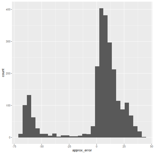
It’s almost never more than .001 in this case.
Interoperability with popular single-cell analysis ecosytems
Seurat
Seurat is an R package designed for QC, analysis, and exploration of single-cell RNA-seq data. Seurat can be used to identify and interpret sources of heterogeneity from single-cell transcriptomic measurements, and to integrate diverse types of single-cell data. Seurat is developed and maintained by the Satija lab and is released under the MIT license.
Although the basic processing of single-cell data with Bioconductor
packages (described in the OSCA book) and
with Seurat is very similar and will produce overall roughly identical
results, there is also complementary functionality with regard to cell
type annotation, dataset integration, and downstream analysis. To make
the most of both ecosystems it is therefore beneficial to be able to
easily switch between a SeuratObject and a
SingleCellExperiment. See also the Seurat conversion
vignette for conversion to/from other popular single cell formats
such as the AnnData format used by scanpy.
Seurat provides helper functions
as.SingleCellExperiment() and as.Seurat() to
convert back and forth between SCEs and Seurat objects.
Scanpy
Scanpy is a scalable toolkit for analyzing single-cell gene expression data built jointly with anndata. It includes preprocessing, visualization, clustering, trajectory inference and differential expression testing. The Python-based implementation efficiently deals with datasets of more than one million cells. Scanpy is developed and maintained by the Theis lab and is released under a BSD-3-Clause license. Scanpy is part of the scverse, a Python-based ecosystem for single-cell omics data analysis.
At the core of scanpy’s single-cell functionality is the
anndata data structure, scanpy’s integrated single-cell
data container, which is conceptually very similar to Bioconductor’s
SingleCellExperiment class.
Bioconductor’s zellkonverter
package provides a lightweight interface between the Bioconductor
SingleCellExperiment data structure and the Python
AnnData-based single-cell analysis environment. The idea is
to enable users and developers to easily move data between these
frameworks to construct a multi-language analysis pipeline across
R/Bioconductor and Python.
R
library(zellkonverter)
The readH5AD() function can be used to read a
SingleCellExperiment from an H5AD file. Here, we use an
example H5AD file contained in the zellkonverter
package.
R
example_h5ad <- system.file("extdata", "krumsiek11.h5ad",
                            package = "zellkonverter")

readH5AD(example_h5ad, reader = "R")
OUTPUT
class: SingleCellExperiment
dim: 11 640
metadata(2): highlights iroot
assays(1): X
rownames(11): Gata2 Gata1 ... EgrNab Gfi1
rowData names(0):
colnames(640): 0 1 ... 158-3 159-3
colData names(1): cell_type
reducedDimNames(0):
mainExpName: NULL
altExpNames(0):
We can also write a SingleCellExperiment to an H5AD file
with the writeH5AD() function. This is demonstrated below
on the wild-type chimera mouse gastrulation dataset.
R
out.file <- tempfile(fileext = ".h5ad")

writeH5AD(sce, file = out.file)
The resulting H5AD file can then be read into Python using scanpy’s read_h5ad function and then directly used in compatible Python-based analysis frameworks.
Exercises
Exercise 1: Out of memory representation
Write the counts matrix of the wild-type chimera mouse gastrulation dataset to an HDF5 file. Create another counts matrix that reads the data from the HDF5 file. Compare memory usage of holding the entire matrix in memory as opposed to holding the data out of memory.
See the HDF5Array function for reading from HDF5 and the
writeHDF5Array function for writing to HDF5 from the HDF5Array
package.
R
wt_out <- tempfile(fileext = ".h5")

wt_counts <- counts(WTChimeraData())
R
writeHDF5Array(wt_counts,
               name = "wt_counts",
               file = wt_out)
OUTPUT
<29453 x 30703> sparse HDF5Matrix object of type "double":
                       cell_1     cell_2     cell_3 ... cell_30702 cell_30703
ENSMUSG00000051951          0          0          0   .          0          0
ENSMUSG00000089699          0          0          0   .          0          0
ENSMUSG00000102343          0          0          0   .          0          0
ENSMUSG00000025900          0          0          0   .          0          0
ENSMUSG00000025902          0          0          0   .          0          0
               ...          .          .          .   .          .          .
ENSMUSG00000095041          0          1          2   .          0          0
ENSMUSG00000063897          0          0          0   .          0          0
ENSMUSG00000096730          0          0          0   .          0          0
ENSMUSG00000095742          0          0          0   .          0          0
         tomato-td          1          0          1   .          0          0
R
oom_wt <- HDF5Array(wt_out, "wt_counts")

object.size(wt_counts)
OUTPUT
1520366960 bytesR
object.size(oom_wt)
OUTPUT
2488 bytesExercise 2: Parallelization
Perform a PCA analysis of the wild-type chimera mouse gastrulation dataset using a multicore backend for parallel computation. Compare the runtime of performing the PCA either in serial execution mode, in multicore execution mode with 2 workers, and in multicore execution mode with 3 workers.
Use the function system.time to obtain the runtime of
each job.
R
sce.brain <- logNormCounts(sce.brain)

system.time({i.out <- runPCA(sce.brain,
                             ncomponents = 20,
                             BSPARAM = ExactParam(),
                             BPPARAM = SerialParam())})

system.time({i.out <- runPCA(sce.brain,
                             ncomponents = 20,
                             BSPARAM = ExactParam(),
                             BPPARAM = MulticoreParam(workers = 2))})

system.time({i.out <- runPCA(sce.brain,
                             ncomponents = 20,
                             BSPARAM = ExactParam(),
                             BPPARAM = MulticoreParam(workers = 3))})
Further Reading
- OSCA book, Chapter 14: Dealing with big data
- The
BiocParallelintro vignette. - Modern Statistics for Modern Biology, Ch. 7 Multivariate Analysis
- Out-of-memory representations can be used to work with single-cell datasets that are too large to fit in memory.
- Parallelization of calculations across genes or cells is an effective strategy for speeding up analysis of large single-cell datasets.
- Fast approximations for nearest neighbor search and singular value composition can speed up essential steps of single-cell analysis with minimal loss of accuracy.
- Converter functions between existing single-cell data formats enable analysis workflows that leverage complementary functionality from poplular single-cell analysis ecosystems.
Session Info
R
sessionInfo()
OUTPUT
R version 4.6.1 (2026-06-24)
Platform: x86_64-pc-linux-gnu
Running under: Linux Mint 22.3

Matrix products: default
BLAS:   /usr/lib/x86_64-linux-gnu/blas/libblas.so.3.12.0
LAPACK: /usr/lib/x86_64-linux-gnu/lapack/liblapack.so.3.12.0  LAPACK version 3.12.0

locale:
 [1] LC_CTYPE=en_US.UTF-8       LC_NUMERIC=C
 [3] LC_TIME=en_US.UTF-8        LC_COLLATE=en_US.UTF-8
 [5] LC_MONETARY=en_US.UTF-8    LC_MESSAGES=en_US.UTF-8
 [7] LC_PAPER=en_US.UTF-8       LC_NAME=C
 [9] LC_ADDRESS=C               LC_TELEPHONE=C
[11] LC_MEASUREMENT=en_US.UTF-8 LC_IDENTIFICATION=C

time zone: America/New_York
tzcode source: system (glibc)

attached base packages:
[1] stats4    stats     graphics  grDevices utils     datasets  methods
[8] base

other attached packages:
 [1] zellkonverter_1.22.0         BiocSingular_1.28.0
 [3] scater_1.40.2                ggplot2_4.0.3
 [5] scuttle_1.22.0               BiocNeighbors_2.6.0
 [7] MouseGastrulationData_1.26.0 SpatialExperiment_1.22.0
 [9] BiocParallel_1.46.0          scrapper_1.6.3
[11] TENxBrainData_1.32.0         HDF5Array_1.40.0
[13] h5mread_1.4.0                rhdf5_2.56.0
[15] DelayedArray_0.38.2          SparseArray_1.12.2
[17] S4Arrays_1.12.0              abind_1.4-8
[19] Matrix_1.7-6                 SingleCellExperiment_1.34.0
[21] SummarizedExperiment_1.42.0  Biobase_2.72.0
[23] GenomicRanges_1.64.0         Seqinfo_1.2.0
[25] IRanges_2.46.0               S4Vectors_0.50.1
[27] BiocGenerics_0.58.1          generics_0.1.4
[29] MatrixGenerics_1.24.0        matrixStats_1.5.0
[31] BiocStyle_2.40.0

loaded via a namespace (and not attached):
 [1] DBI_1.3.0            formatR_1.14         gridExtra_2.3.1
 [4] httr2_1.3.0          rlang_1.3.0          magrittr_2.0.5
 [7] otel_0.2.0           compiler_4.6.1       RSQLite_3.53.3
[10] dir.expiry_1.20.0    png_0.1-9            vctrs_0.7.3
[13] pkgconfig_2.0.3      crayon_1.5.3         fastmap_1.2.0
[16] dbplyr_2.6.0         magick_2.9.1         XVector_0.52.0
[19] labeling_0.4.3       rmarkdown_2.31       ggbeeswarm_0.7.3
[22] purrr_1.2.2          bit_4.6.0            xfun_0.60
[25] cachem_1.1.0         beachmat_2.28.0      jsonlite_2.0.0
[28] blob_1.3.0           rhdf5filters_1.24.1  Rhdf5lib_2.0.0
[31] irlba_2.3.7          parallel_4.6.1       R6_2.6.1
[34] RColorBrewer_1.1-3   reticulate_1.46.0    Rcpp_1.1.2
[37] knitr_1.51           tidyselect_1.2.1     viridis_0.6.5
[40] rstudioapi_0.19.0    yaml_2.3.12          codetools_0.2-20
[43] curl_7.1.0           lattice_0.22-9       tibble_3.3.1
[46] withr_3.0.3          KEGGREST_1.52.2      BumpyMatrix_1.20.0
[49] S7_0.2.2             evaluate_1.0.5       BiocFileCache_3.2.0
[52] ExperimentHub_3.2.0  Biostrings_2.80.1    pillar_1.11.1
[55] BiocManager_1.30.27  filelock_1.0.3       renv_1.2.3
[58] BiocVersion_3.23.1   scales_1.4.0         glue_1.8.1
[61] tools_4.6.1          AnnotationHub_4.2.2  ScaledMatrix_1.20.0
[64] grid_4.6.1           AnnotationDbi_1.74.0 basilisk_1.24.0
[67] beeswarm_0.4.0       vipor_0.4.7          rsvd_1.0.5
[70] cli_3.6.6            rappdirs_0.3.4       viridisLite_0.4.3
[73] dplyr_1.2.1          gtable_0.3.6         digest_0.6.39
[76] ggrepel_0.9.8        rjson_0.2.23         farver_2.1.2
[79] memoise_2.0.1        htmltools_0.5.9      lifecycle_1.0.5
[82] httr_1.4.8           bit64_4.8.2