Conformal Prediction for cell type annotation
Daniela Corbetta
Department of Statistical Sciences, University of Padovadaniela.corbetta@unipd.it Source:
vignettes/scConform.Rmd
scConform.RmdIntroduction
Cell type annotation is a crucial step in bioinformatic research. A multitude of annotated datasets are now readily accessible, providing valuable references for annotating cells in unannotated datasets originating from similar tissues. Typically, a model is chosen and trained on the reference data to predict the label of a new, unannotated cell in the query dataset.
These methods commonly provide point predictions of the cell label,
along with estimated probabilities or scores assigned to each cell type
in the reference dataset. However, relying solely on point predictions
can be problematic when the corresponding estimated probability is low,
leading to unreliable classification. To address this issue, we propose
to exploit conformal inference to return prediction sets that include
multiple labels, with the set size reflecting the confidence in the
point prediction. The package scConform implements two
methods to achieve this:
The first method uses split conformal inference (as a reference, see for example section 1 of Angelopoulus and Bates, 2022). The output is a prediction set, , that contains some of the cell types present in the reference data. Let be the true cell type of a new cell in the query dataset. Then, satisfies , where is a user-chosen error level.
The second method is based on conformal risk control (Angelopoulus et al., 2023). It considers the inherent relationships among cell types that are encoded as graph-structured constraints available through the cell ontology. The final output is a prediction set aligned with the cell ontology structure. Specifically, the prediction set will include all the children of an ancestor of the predicted class. The more unsure the point prediction, the broader the classification. Also this method satisfies . More details are available at Corbetta et al., 2026+.
Installation
To install it
if (BiocManager::version() >= "3.23") {
    BiocManager::install("scConform")
} else {
    spdl::info(
        "'scConform' requires Bioconductor version 3.23 or later, ",
        "installing development version from Github"
    )
    devtools::install_github("ccb-hms/scConform")
}
Preliminaries
Load data and cell ontology
As an example, we’ll use the mouse ileum Merfish data from the
MerfishData Bioconductor package, segmented with Baysor.
For the purpose of this vignette, we’ll treat the data as if they were
single-cell data, discarding the spatial information. This is a toy
example in which reference and query data will be a subset of the same
dataset. In real life examples, data integration is a necessary first
step.
Next, load the cell ontology trough the ontoProc
Bioconductor package.
# Load data
spe_baysor <- MouseIleumPetukhov2021(
    segmentation = "baysor",
    use.images = FALSE, use.polygons = FALSE
)
# Load ontology
cl <- getOnto("cellOnto", "2023")
#> loading from cache
Build the ontology
The object cl contains information regarding all the
relationships among all the known cell types. The first step is to
filter the ontology and only keep the parts related to the cell types
that are present in the data.
This dataset does not provide annotations with the cell ontology tags, so we need to browse the ontology to find the interesting tags.
For more information on how to restrict the cell ontology, refer to the ontoProc documentation.
tags <- c(
    "CL:0009022", # Stromal
    "CL:0000236", # B cell
    "CL:0009080", # Tuft
    "CL:1000411", # Endothelial
    "CL:1000335", # Enterocyte
    "CL:1000326", # Goblet
    "CL:0002088", # ICC
    "CL:0009007", # Macrophage + DC
    "CL:1000343", # Paneth
    "CL:0000669", # Pericyte
    "CL:1000278", # Smooth Muscle
    "CL:0009017", # Stem + TA
    "CL:0000492", # T (CD4+)
    "CL:0000625", # T (CD8+)
    "CL:0017004" # Telocyte
)
opi <- graph_from_graphnel(onto_plot2(cl, tags))
In the opi object, there are also instances from other
ontologies (CARO and BFO) that need to be removed.
Moreover, the names of the leaf nodes of the ontology must correspond to the names used for the annotation.
## Delete CARO and BFO instances
sel_ver <- V(opi)$name[c(grep("CARO", V(opi)$name), grep("BFO", V(opi)$name))]
opi1 <- opi - sel_ver

## Rename vertex to match annotations
V(opi1)$name[grep("CL:0000236", V(opi1)$name)] <- "B cell"
V(opi1)$name[grep("CL:1000411", V(opi1)$name)] <- "Endothelial"
V(opi1)$name[grep("CL:1000335", V(opi1)$name)] <- "Enterocyte"
V(opi1)$name[grep("CL:1000326", V(opi1)$name)] <- "Goblet"
V(opi1)$name[grep("CL:0002088", V(opi1)$name)] <- "ICC"
V(opi1)$name[grep("CL:0009007", V(opi1)$name)] <- "Macrophage + DC"
V(opi1)$name[grep("CL:1000343", V(opi1)$name)] <- "Paneth"
V(opi1)$name[grep("CL:0000669", V(opi1)$name)] <- "Pericyte"
V(opi1)$name[grep("CL:1000278", V(opi1)$name)] <- "Smooth Muscle"
V(opi1)$name[grep("CL:0009017", V(opi1)$name)] <- "Stem + TA"
V(opi1)$name[grep("CL:0009022", V(opi1)$name)] <- "Stromal"
V(opi1)$name[grep("CL:0000492", V(opi1)$name)] <- "T (CD4+)"
V(opi1)$name[grep("CL:0000625", V(opi1)$name)] <- "T (CD8+)"
V(opi1)$name[grep("CL:0017004", V(opi1)$name)] <- "Telocyte"
V(opi1)$name[grep("CL:0009080", V(opi1)$name)] <- "Tuft"

## Add the edge from connective tissue cell and telocyte and delete redundant
## nodes
opi1 <- add_edges(opi1, c("connective\ntissue cell\nCL:0002320", "Telocyte"))
gr <- as_graphnel(opi1)
opi2 <- opi1 - c(
    "somatic\ncell\nCL:0002371", "contractile\ncell\nCL:0000183",
    "native\ncell\nCL:0000003"
)


V(opi2)$name <- trimws(gsub("CL:.*|\\n", " ", V(opi2)$name))

gr1 <- as_graphnel(opi2)

## Plot the final ontology
attrs <- list(node = list(shape = "box", fontsize = 15, fixedsize = FALSE))
plot(gr1, attrs = attrs)
Preprocess data
Modify the colData variable leiden_final to unify B
cells and enterocytes
spe_baysor$cell_type <- spe_baysor$leiden_final
spe_baysor$cell_type[spe_baysor$cell_type %in% c(
    "B (Follicular, Circulating)",
    "B (Plasma)"
)] <- "B cell"
spe_baysor$cell_type[grep("Enterocyte", spe_baysor$cell_type)] <- "Enterocyte"
spe_baysor <- spe_baysor[, spe_baysor$cell_type %notin% c(
    "Removed",
    "Myenteric Plexus"
)]
spe_baysor
#> class: SpatialExperiment
#> dim: 241 5163
#> metadata(0):
#> assays(2): counts molecules
#> rownames(241): Acsl1 Acta2 ... Vcan Vim
#> rowData names(0):
#> colnames: NULL
#> colData names(8): n_transcripts density ... sample_id cell_type
#> reducedDimNames(0):
#> mainExpName: NULL
#> altExpNames(0):
#> spatialCoords names(2) : x y
#> imgData names(1): sample_id

# See frequencies of cell types
table(spe_baysor$cell_type)
#>
#>          B cell     Endothelial      Enterocyte          Goblet             ICC
#>             536             231            1257             299              31
#> Macrophage + DC          Paneth        Pericyte   Smooth Muscle       Stem + TA
#>             427             328             102             428             580
#>         Stromal        T (CD4+)        T (CD8+)        Telocyte            Tuft
#>             489             197             125             115              18
Now randomly split the data into reference and query data.
set.seed(1636)
ref <- sample(seq_len(ncol(spe_baysor)), 600)

spe_ref <- spe_baysor[, ref]
spe_query <- spe_baysor[, -ref]
# Reference data
spe_ref
#> class: SpatialExperiment
#> dim: 241 600
#> metadata(0):
#> assays(2): counts molecules
#> rownames(241): Acsl1 Acta2 ... Vcan Vim
#> rowData names(0):
#> colnames: NULL
#> colData names(8): n_transcripts density ... sample_id cell_type
#> reducedDimNames(0):
#> mainExpName: NULL
#> altExpNames(0):
#> spatialCoords names(2) : x y
#> imgData names(1): sample_id
# Query data
spe_query
#> class: SpatialExperiment
#> dim: 241 4563
#> metadata(0):
#> assays(2): counts molecules
#> rownames(241): Acsl1 Acta2 ... Vcan Vim
#> rowData names(0):
#> colnames: NULL
#> colData names(8): n_transcripts density ... sample_id cell_type
#> reducedDimNames(0):
#> mainExpName: NULL
#> altExpNames(0):
#> spatialCoords names(2) : x y
#> imgData names(1): sample_id
Fit a classification model
We now need to build a classification model. To this aim, we’ll draw a random sample of 300 cells from the reference data, and train a multinomial model on those. As explanatory variables we’ll use the 50 most variable genes. For this step, every statistical model or machine learning method can be used, as long as it provides also estimated probabilities for each class.
# Randomly select 300 cells
set.seed(1704)
train <- sample(seq_len(ncol(spe_ref)), 300)
# Training data
spe_train <- spe_ref[, train]
spe_train
#> class: SpatialExperiment
#> dim: 241 300
#> metadata(0):
#> assays(2): counts molecules
#> rownames(241): Acsl1 Acta2 ... Vcan Vim
#> rowData names(0):
#> colnames: NULL
#> colData names(8): n_transcripts density ... sample_id cell_type
#> reducedDimNames(0):
#> mainExpName: NULL
#> altExpNames(0):
#> spatialCoords names(2) : x y
#> imgData names(1): sample_id

# get HVGs
spe_train <- logNormCounts(spe_train)
v <- modelGeneVar(spe_train)
hvg <- getTopHVGs(v, n = 50)

# Extract counts and convert data into a data.frame format
df_train <- as.data.frame(t(as.matrix(counts(spe_train[hvg, ]))))
df_train$Y <- spe_train$cell_type
table(df_train$Y)
#>
#>          B cell     Endothelial      Enterocyte          Goblet             ICC
#>              25              10              68              19               2
#> Macrophage + DC          Paneth        Pericyte   Smooth Muscle       Stem + TA
#>              28              17               4              22              48
#>         Stromal        T (CD4+)        T (CD8+)        Telocyte            Tuft
#>              34              13               5               4               1

# Fit multinomial model
fit <- vglm(Y ~ .,
    family = multinomial(refLevel = "B cell"),
    data = df_train
)
Method 1: standard conformal inference
Algorithm
As anticipated in the introduction, the first method uses split conformal inference to build the prediction sets. It requires to split the reference data into two subsets:
- training set: portion of the reference data to be used to build a classifier (the multinomial model in our example)
- calibration set: portion of the reference data to be used to calibrate the procedure.
Given and the calibration data, the objective of conformal inference is to build, for a new non-annotated cell , a prediction set that satisfies
where is the true label of the new cell and is a user-chosen error level. The algorithm for split conformal inference is the following:
For the data in the calibration set, obtain the conformal scores (i.e. 1 minus the estimated probability that the model is assigning to the true label of the -th cell). These scores will be high when the model is assigning a small probability to the true class, and low otherwise.
Obtain as the empirical quantile of the conformal scores.
Finally, for a new cell , build a prediction set by including all the classes or which the estimated probability is higher than :
Obtain prediction matrices
The first step to build conformal prediction sets is to obtain matrices with the estimated probabilities for each cell type for cells in the calibration data and in the query data. Each row of the matrix corresponds to a particular cell, while each row to a different cell type. The entry of the matrix indicates the estimated probability that the cell is of type .
spe_cal <- spe_ref[, -train]
# Prediction matrix for calibration data
df_cal <- as.data.frame(t(as.matrix(counts(spe_cal[hvg, ]))))
p_cal <- predict(fit, newdata = df_cal, type = "response")
head(round(p_cal, 3))
#>   B cell Endothelial Enterocyte Goblet   ICC Macrophage + DC Paneth Pericyte
#> 1  0.001       0.000      0.023  0.000 0.000           0.561  0.000    0.000
#> 2  0.000       0.000      0.000  0.000 0.000           0.000  0.000    0.000
#> 3  0.018       0.000      0.041  0.000 0.001           0.923  0.000    0.001
#> 4  0.001       0.001      0.283  0.035 0.001           0.003  0.017    0.000
#> 5  0.000       0.000      1.000  0.000 0.000           0.000  0.000    0.000
#> 6  0.000       0.000      0.002  0.000 0.000           0.000  0.141    0.000
#>   Smooth Muscle Stem + TA Stromal T (CD4+) T (CD8+) Telocyte  Tuft
#> 1         0.002     0.000   0.407    0.000    0.000    0.006 0.000
#> 2         0.000     0.000   0.000    0.001    0.999    0.000 0.000
#> 3         0.005     0.007   0.001    0.001    0.000    0.000 0.001
#> 4         0.004     0.161   0.488    0.001    0.002    0.003 0.001
#> 5         0.000     0.000   0.000    0.000    0.000    0.000 0.000
#> 6         0.000     0.856   0.000    0.000    0.000    0.000 0.000
# Prediction matrix for query data
df_test <- as.data.frame(t(as.matrix(counts(spe_query[hvg, ]))))
p_test <- predict(fit, newdata = df_test, type = "response")
head(round(p_test, 3))
#>   B cell Endothelial Enterocyte Goblet ICC Macrophage + DC Paneth Pericyte
#> 1      0       0.627          0      0   0               0      0        0
#> 2      0       0.000          0      0   0               0      0        0
#> 3      0       0.001          0      0   0               0      0        0
#> 4      0       0.000          0      0   0               0      0        0
#> 5      0       0.000          0      0   0               0      0        0
#> 6      0       0.000          0      0   0               0      0        0
#>   Smooth Muscle Stem + TA Stromal T (CD4+) T (CD8+) Telocyte Tuft
#> 1         0.000         0   0.001    0.000        0    0.372    0
#> 2         0.997         0   0.000    0.000        0    0.003    0
#> 3         0.021         0   0.002    0.001        0    0.975    0
#> 4         1.000         0   0.000    0.000        0    0.000    0
#> 5         0.930         0   0.069    0.000        0    0.001    0
#> 6         1.000         0   0.000    0.000        0    0.000    0
Obtain conformal prediction sets
We can now directly call the getPredictionSet function
by using as input the prediction matrices for the calibration and the
query dataset. In this case, the output of the function will be a list
whose elements are the prediction sets for each query cell.
By setting follow_ontology=FALSE, we are asking the
function to return prediction sets obtained via split conformal
inference. The parameter onto is not necessary with this
method, but if the ontology is provided then it will be used by the
function to retrieve the considered cell types. Alternatively, we can
explicitly provide the labels with the parameter labels.
The parameter alpha indicates the allowed miscoverage
percentage. For example, if we set alpha=0.1, it means that
at most 10% of the prediction sets we obtain will not include the true
label.
labels <- colnames(p_test)
sets <- getPredictionSets(
    x_query = p_test,
    x_cal = p_cal,
    y_cal = spe_cal$cell_type,
    alpha = 0.1,
    follow_ontology = FALSE,
    labels = labels
)

# See the first six prediction sets
sets[1:6]
#> [[1]]
#> [1] "Endothelial" "Telocyte"
#>
#> [[2]]
#> [1] "Smooth Muscle"
#>
#> [[3]]
#> [1] "Smooth Muscle" "Telocyte"
#>
#> [[4]]
#> [1] "Smooth Muscle"
#>
#> [[5]]
#> [1] "Smooth Muscle" "Stromal"
#>
#> [[6]]
#> [1] "Smooth Muscle"
Since in this example the cell labels are available, we can
explicitly check that the constraint on the miscoverage is satisfied by
computing the proportion of sets that include the true label. We set
alpha=0.1, so we expect this proportion to be higher than
0.9.
# Check coverage
cvg <- rep(NA, length(sets))
for (i in seq_len(length(sets))) {
    cvg[i] <- spe_query$cell_type[i] %in% sets[[i]]
}
mean(cvg)
#> [1] 0.9035722
As an alternative, we can provide as input a
SingleCellExperiment object. In this case, it needs to have
the estimated probabilities for each cell type in the
colData. The names of these colData have to
correspond to the names of the leaf nodes in the ontology.
The output will be a SingleCellExperiment object with a
new variable in the colData containing the prediction sets.
The name of this variable can be assigned trough the
pr_name parameter.
# Retrieve labels as leaf nodes of the ontology
labels <- V(opi2)$name[degree(opi2, mode = "out") == 0]

# Create corresponding colData
for (i in labels) {
    colData(spe_cal)[[i]] <- p_cal[, i]
    colData(spe_query)[[i]] <- p_test[, i]
}

# Create prediction sets
spe_query <- getPredictionSets(
    x_query = spe_query,
    x_cal = spe_cal,
    y_cal = spe_cal$cell_type,
    alpha = 0.1,
    follow_ontology = FALSE,
    pr_name = "pred_set",
    labels = labels
)

# See the new variable pred_set into the colData
head(colData(spe_query))
#> DataFrame with 6 rows and 24 columns
#>   n_transcripts   density elongation      area avg_confidence  leiden_final
#>       <numeric> <numeric>  <numeric> <numeric>      <numeric>   <character>
#> 1            39   0.02159      5.082      1806         0.8647   Endothelial
#> 2           165   0.02016      1.565      8186         0.9528 Smooth Muscle
#> 3           139   0.02279      1.820      6100         0.9762 Smooth Muscle
#> 4            80   0.01828      1.546      4376         0.9076 Smooth Muscle
#> 5            75   0.02479      3.475      3025         0.8952 Smooth Muscle
#> 6           167   0.02409      1.265      6932         0.9618 Smooth Muscle
#>     sample_id     cell_type     Stromal      B cell        Tuft Endothelial
#>   <character>   <character>   <numeric>   <numeric>   <numeric>   <numeric>
#> 1       ileum   Endothelial 1.06770e-03 4.62746e-06 1.09285e-06 6.26716e-01
#> 2       ileum Smooth Muscle 2.48790e-07 2.11623e-12 1.71646e-09 4.27276e-13
#> 3       ileum Smooth Muscle 1.82261e-03 1.05365e-06 3.42260e-05 1.45712e-03
#> 4       ileum Smooth Muscle 4.46595e-07 8.68709e-12 1.84782e-10 1.48018e-11
#> 5       ileum Smooth Muscle 6.87351e-02 5.40229e-05 3.80670e-05 1.56797e-04
#> 6       ileum Smooth Muscle 6.47366e-15 2.80039e-21 2.51182e-16 3.76540e-21
#>    Enterocyte      Goblet         ICC Macrophage + DC      Paneth    Pericyte
#>     <numeric>   <numeric>   <numeric>       <numeric>   <numeric>   <numeric>
#> 1 6.23838e-09 2.16089e-06 1.04065e-04     8.69702e-11 2.46469e-08 1.25208e-06
#> 2 3.65028e-15 5.45567e-19 3.26311e-10     3.71068e-15 1.04596e-11 7.83728e-11
#> 3 7.62737e-11 1.02715e-10 1.30690e-04     4.16898e-09 1.48191e-07 2.69325e-06
#> 4 3.06169e-10 4.21061e-16 8.73496e-10     1.02177e-11 3.33635e-09 1.75309e-11
#> 5 9.53445e-06 1.14109e-06 1.68140e-05     3.24168e-06 3.04576e-04 4.81784e-06
#> 6 1.27740e-21 9.27025e-38 7.72260e-16     3.18369e-21 1.04362e-26 5.48492e-22
#>   Smooth Muscle   Stem + TA    T (CD4+)    T (CD8+)    Telocyte
#>       <numeric>   <numeric>   <numeric>   <numeric>   <numeric>
#> 1   3.17594e-12 1.94285e-04 2.61437e-07 1.10020e-05 3.71897e-01
#> 2   9.97273e-01 4.23329e-18 3.08082e-10 4.01534e-10 2.72648e-03
#> 3   2.11629e-02 5.03876e-11 5.90176e-04 2.05918e-05 9.74778e-01
#> 4   9.99986e-01 5.59105e-10 4.55175e-09 9.09174e-10 1.35576e-05
#> 5   9.29946e-01 5.76652e-07 5.48474e-05 1.91186e-05 6.55575e-04
#> 6   9.99984e-01 1.63394e-24 1.70917e-14 4.89589e-15 1.60623e-05
#>                 pred_set
#>                   <list>
#> 1   Endothelial,Telocyte
#> 2          Smooth Muscle
#> 3 Smooth Muscle,Telocyte
#> 4          Smooth Muscle
#> 5  Stromal,Smooth Muscle
#> 6          Smooth Muscle
Method 2: exploit the cell ontology
Algorithm
Let be the class with the maximum estimated probability. Moreover, given a directed graph let and be the set of children nodes and ancestor nodes of , respectively. Finally, for each node define a score as the sum of the predicted probabilities of the leaf nodes that are children of . We build the sets as follows:
where and .
In words, we start from the predicted class and we go up in the graph until we find an ancestor of that has a score that is at least and include in the prediction sets all its children. Then we add to this subgraph the other ones that contain for which the score is less than . To choose , we follow eq. (4) in Angelopoulus et al., 2023, considering the miscoverage as loss function. See Corbetta et al., 2026+ for more details on the algorithm and a discussion on the rationale of the method.
Obtain hierarchical prediction sets
To switch to the hierarchical algorithm, we just need to set
follow_ontology=TRUE and provide an ontology to the
onto parameter. As in the previous case, if the input is a
SingleCellExperiment object then the output will be again a
SingleCellExperiment object with a new variable containing
the prediction sets in the colData.
spe_query <- getPredictionSets(
    x_query = spe_query,
    x_cal = spe_cal,
    y_cal = spe_cal$cell_type,
    onto = opi2,
    alpha = 0.1,
    follow_ontology = TRUE,
    method = "full",
    pr_name = "pred_set_hier",
    BPPARAM = MulticoreParam(workers = 2),
    simplify = FALSE
)
#> Calibration complete. Selected lambda_hat = 0.908272727272727

# See the first six prediction sets
head(spe_query$pred_set_hier)
#> [[1]]
#>  [1] "Tuft"            "Endothelial"     "Enterocyte"      "Goblet"
#>  [5] "ICC"             "Paneth"          "Stem + TA"       "Stromal"
#>  [9] "B cell"          "Macrophage + DC" "Pericyte"        "Smooth Muscle"
#> [13] "T (CD4+)"        "T (CD8+)"        "Telocyte"
#>
#> [[2]]
#> [1] "Smooth Muscle"
#>
#> [[3]]
#> [1] "Telocyte"
#>
#> [[4]]
#> [1] "Smooth Muscle"
#>
#> [[5]]
#> [1] "Smooth Muscle"
#>
#> [[6]]
#> [1] "Smooth Muscle"
Also in this case, we can check the coverage:
# Check coverage
cvg1 <- rep(NA, length(spe_query$pred_set_hier))
for (i in seq_len(length(spe_query$pred_set_hier))) {
    cvg1[i] <- spe_query$cell_type[i] %in% spe_query$pred_set_hier[[i]]
}

mean(cvg1)
#> [1] 0.8912996
As an alternative, we can choose to return only the common ancestor,
instead of the entire set of predicted labels. This can be done directly
in the function by setting simplify=TRUE. Alternatively, we
can convert the obtained prediction sets invoking the function
getCommonAncestor.
spe_query$pred_set_hier_simp <- vapply(
    spe_query$pred_set_hier,
    function(x) getCommonAncestor(x, opi2),
    character(1)
)
head(spe_query$pred_set_hier_simp)
#> [1] "animal cell"   "Smooth Muscle" "Telocyte"      "Smooth Muscle"
#> [5] "Smooth Muscle" "Smooth Muscle"
Visualization
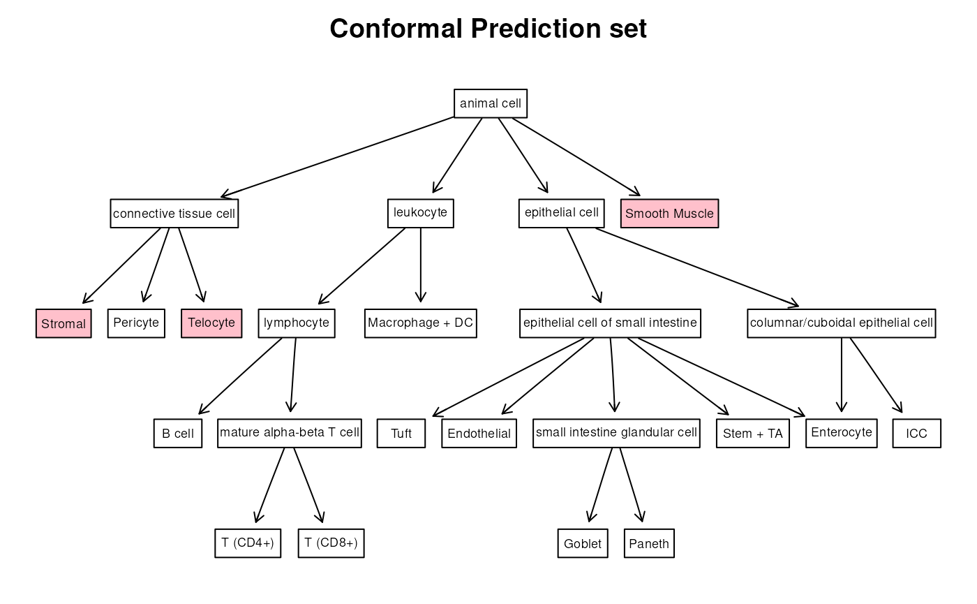
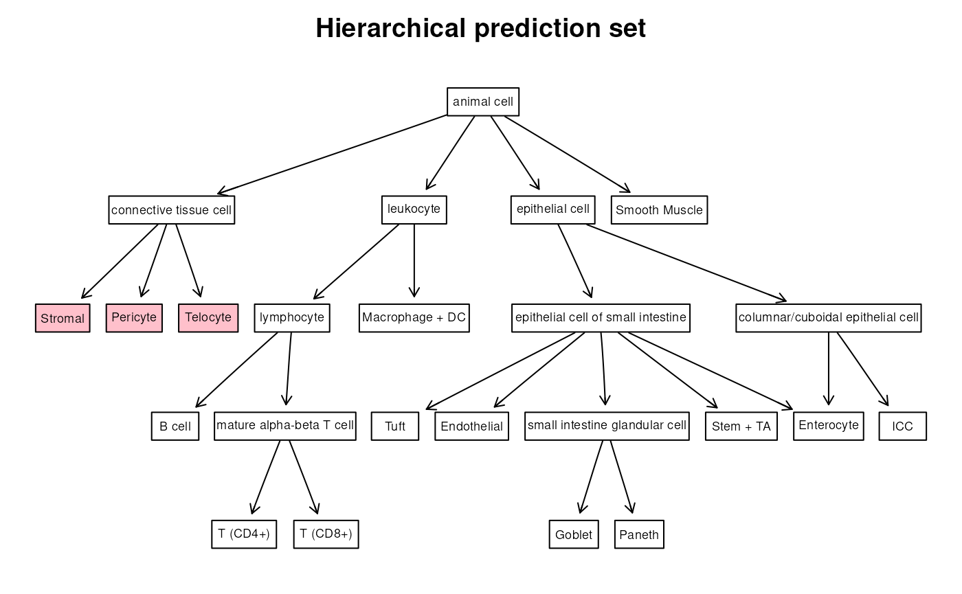
Let’s now visualize the obtained prediction sets. The simplest way is to just ask to color the labels included in the prediction set. Let’s compare the prediction sets for one cell obtained with the two methods
plotResult(spe_query$pred_set[[75]], opi2,
    col_grad = "pink", attrs = attrs, add_scores = FALSE,
    title = "Conformal Prediction set"
)
plotResult(spe_query$pred_set_hier[[75]], opi2,
    col_grad = "pink", attrs = attrs, add_scores = FALSE,
    title = "Hierarchical prediction set"
)
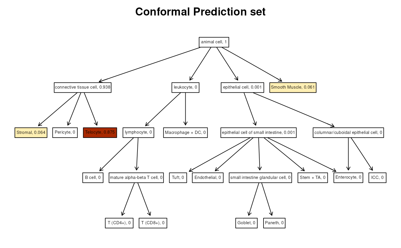
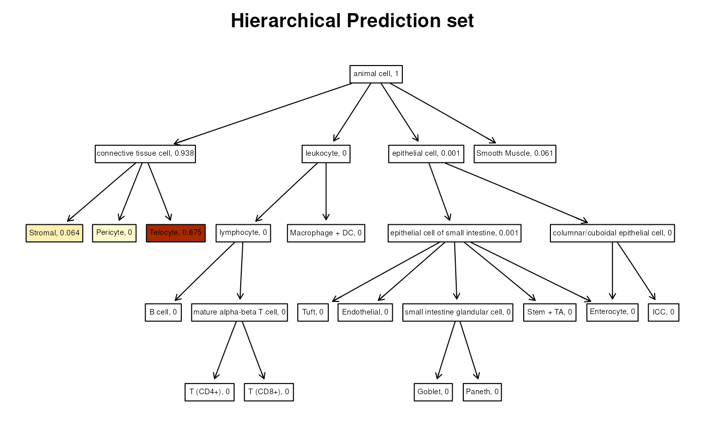
We can now instead give as input also the estimated probabilities and
a gradient. The function will color the cells according to the gradient,
with stronger colors corresponding to higher probabilities. If
add_scores=TRUE, then the estimated probabilities will be
added to the labels.
plotResult(spe_query$pred_set[[75]], opi2,
    probs = p_test[75, ],
    col_grad = c("lemonchiffon", "orange", "darkred"),
    attrs = attrs, add_scores = TRUE,
    title = "Conformal Prediction set"
)
plotResult(spe_query$pred_set_hier[[75]], opi2,
    probs = p_test[75, ],
    col_grad = c("lemonchiffon", "orange", "darkred"),
    attrs = attrs, add_scores = TRUE,
    title = "Hierarchical Prediction set"
)
R.session Info
R version 4.5.2 (2025-10-31)
Platform: x86_64-pc-linux-gnu
Running under: Ubuntu 24.04.3 LTS

Matrix products: default
BLAS:   /usr/lib/x86_64-linux-gnu/openblas-pthread/libblas.so.3
LAPACK: /usr/lib/x86_64-linux-gnu/openblas-pthread/libopenblasp-r0.3.26.so;  LAPACK version 3.12.0

locale:
 [1] LC_CTYPE=en_US.UTF-8       LC_NUMERIC=C
 [3] LC_TIME=en_US.UTF-8        LC_COLLATE=en_US.UTF-8
 [5] LC_MONETARY=en_US.UTF-8    LC_MESSAGES=en_US.UTF-8
 [7] LC_PAPER=en_US.UTF-8       LC_NAME=C
 [9] LC_ADDRESS=C               LC_TELEPHONE=C
[11] LC_MEASUREMENT=en_US.UTF-8 LC_IDENTIFICATION=C

time zone: UTC
tzcode source: system (glibc)

attached base packages:
[1] splines   stats4    stats     graphics  grDevices utils     datasets
[8] methods   base

other attached packages:
 [1] BiocParallel_1.44.0         scran_1.38.0
 [3] scuttle_1.20.0              igraph_2.2.1
 [5] MerfishData_1.12.0          SpatialExperiment_1.20.0
 [7] EBImage_4.52.0              ontoProc_2.4.0
 [9] ontologyIndex_2.12          VGAM_1.1-14
[11] SingleCellExperiment_1.32.0 SummarizedExperiment_1.40.0
[13] Biobase_2.70.0              GenomicRanges_1.62.1
[15] Seqinfo_1.0.0               IRanges_2.44.0
[17] S4Vectors_0.48.0            BiocGenerics_0.56.0
[19] generics_0.1.4              MatrixGenerics_1.22.0
[21] matrixStats_1.5.0           scConform_0.99.1
[23] BiocStyle_2.38.0

loaded via a namespace (and not attached):
  [1] jsonlite_2.0.0       magrittr_2.0.4       magick_2.9.0
  [4] rmarkdown_2.30       fs_1.6.6             ragg_1.5.0
  [7] vctrs_0.7.1          memoise_2.0.1        ellmer_0.4.0
 [10] RCurl_1.98-1.17      htmltools_0.5.9      S4Arrays_1.10.1
 [13] AnnotationHub_4.0.0  curl_7.0.0           BiocNeighbors_2.4.0
 [16] Rhdf5lib_1.32.0      SparseArray_1.10.8   rhdf5_2.54.1
 [19] sass_0.4.10          bslib_0.10.0         htmlwidgets_1.6.4
 [22] desc_1.4.3           httr2_1.2.2          cachem_1.1.0
 [25] mime_0.13            lifecycle_1.0.5      pkgconfig_2.0.3
 [28] rsvd_1.0.5           Matrix_1.7-4         R6_2.6.1
 [31] fastmap_1.2.0        shiny_1.12.1         digest_0.6.39
 [34] AnnotationDbi_1.72.0 dqrng_0.4.1          irlba_2.3.7
 [37] ExperimentHub_3.0.0  textshaping_1.0.4    RSQLite_2.4.6
 [40] beachmat_2.26.0      filelock_1.0.3       httr_1.4.7
 [43] abind_1.4-8          compiler_4.5.2       withr_3.0.2
 [46] bit64_4.6.0-1        S7_0.2.1             tiff_0.1-12
 [49] DBI_1.2.3            HDF5Array_1.38.0     rappdirs_0.3.4
 [52] DelayedArray_0.36.0  rjson_0.2.23         bluster_1.20.0
 [55] tools_4.5.2          otel_0.2.0           httpuv_1.6.16
 [58] glue_1.8.0           h5mread_1.2.1        rhdf5filters_1.22.0
 [61] promises_1.5.0       grid_4.5.2           cluster_2.1.8.2
 [64] metapod_1.18.0       BiocSingular_1.26.1  ScaledMatrix_1.18.0
 [67] XVector_0.50.0       BiocVersion_3.22.0   pillar_1.11.1
 [70] limma_3.66.0         BumpyMatrix_1.18.0   later_1.4.5
 [73] dplyr_1.2.0          BiocFileCache_3.0.0  lattice_0.22-9
 [76] bit_4.6.0            tidyselect_1.2.1     RBGL_1.86.0
 [79] coro_1.1.0           locfit_1.5-9.12      Biostrings_2.78.0
 [82] knitr_1.51           bookdown_0.46        edgeR_4.8.2
 [85] ontologyPlot_1.7     xfun_0.56            statmod_1.5.1
 [88] DT_0.34.0            fftwtools_0.9-11     paintmap_1.0
 [91] yaml_2.3.12          evaluate_1.0.5       codetools_0.2-20
 [94] tibble_3.3.1         Rgraphviz_2.54.0     BiocManager_1.30.27
 [97] graph_1.88.1         cli_3.6.5            xtable_1.8-4
[100] reticulate_1.44.1    systemfonts_1.3.1    jquerylib_0.1.4
[103] Rcpp_1.1.1           dbplyr_2.5.1         png_0.1-8
[106] parallel_4.5.2       pkgdown_2.2.0        blob_1.3.0
[109] jpeg_0.1-11          bitops_1.0-9         purrr_1.2.1
[112] crayon_1.5.3         rlang_1.1.7          KEGGREST_1.50.0