re_results <- calculateReconstructionError(
    reference_data = ref_sce,
    query_data = query_sce,
    ref_cell_type_col = "true_cell_type",
    query_cell_type_col = "SingleR_annotation",
    cell_types = "pyramidal CA1",
    pc_subset = 1:5,
    n_hvgs = 100,
    mad_multiplier = 2
)Zeisel Mouse Brain Benchmarking
Overview
This page demonstrates a rigorous quantitative benchmarking of scDiagnostics using the well-characterized Zeisel mouse brain scRNA-seq dataset. To evaluate how our diagnostic tools perform under the realistic complexities of single-cell label transfer, we systematically withheld specific cell populations from the reference to simulate unrepresented biological states.
We then stress-tested the anomaly detection methods against gradients of technical and biological confounders: label noise, class imbalance, and simulated batch effects.
Dataset Context
- Dataset:
scRNAseq::ZeiselBrainData()(3,005 cells, 20,006 genes) - Reference Generation: A 70% split of the dataset serving as the reference atlas.
- Query Generation: The remaining 30% serving as the query dataset. Annotations were transferred using SingleR.
- Hidden Cell States: To simulate missing biological populations, we selectively removed:
- A distinct lineage (Astrocytes)
- A closely related subtype (Pyramidal SS hidden, Pyramidal CA1 present)
- A rare population (Microglia)
1. Benchmarking Framework & Results
Script: R/brain/Supplementary_Figure_1-4.R
To benchmark the detection performance of both the Isolation Forest and Reconstruction Error algorithms, we mapped query cells to the reference and tracked AUROC, AUPRC, Sensitivity, and Specificity across varying degrees of data distortion.
Ground Truth Manifold & AUROC

A) Ground Truth Manifold: A UMAP embedding highlighting the test populations. The Reference (Pyramidal CA1) is shown in blue. The withheld states vary in their transcriptomic distance from this reference (Related, Rare, Distinct).
B) Baseline Detection Accuracy: Both Isolation Forest and Reconstruction Error easily identify missing cell states under clean, ideal conditions, achieving near-perfect AUROC regardless of whether the missing state is closely related, rare, or entirely distinct.
C-H) Stress Testing (Gradients):
- Label Noise: We randomly shuffled 0% to 40% of the reference labels. Anomaly detection remains remarkably stable even up to 20% noise.
- Class Imbalance: We downsampled the reference population from 300 cells down to 10.
scDiagnosticsmaintains high detection power even when the reference representation is extremely sparse. - Batch Effects: We introduced simulated log-count shifts (0 to +2.0). As batch effects become severe, Reconstruction Error begins to degrade faster than Isolation Forest, highlighting Isolation Forest as a highly robust choice for non-ideal integrations.
Note: Companion figures detailing AUPRC, Sensitivity, and Specificity can be generated locally by running the R/brain/Supplementary_Figure_1-4.R script.
NoteFunction Details: calculateReconstructionError()
Parameters:
reference_data,query_data— SCE objects to comparecell_types— Specific reference cell type cluster to build the PCA space uponpc_subset— Subspace dimensionality used for reconstructionn_hvgs— Number of highly variable genes used for local feature selectionmad_multiplier— Adaptive thresholding parameter determining how many Median Absolute Deviations (MADs) above the reference median constitutes an anomaly.
2. Hyperparameter Tuning
To provide practical guidance to users, we systematically evaluated hyperparameter grids for both algorithms to understand the trade-offs between Sensitivity and Specificity.
Isolation Forest Tuning
Script: R/brain/Supplementary_Figure_5.R
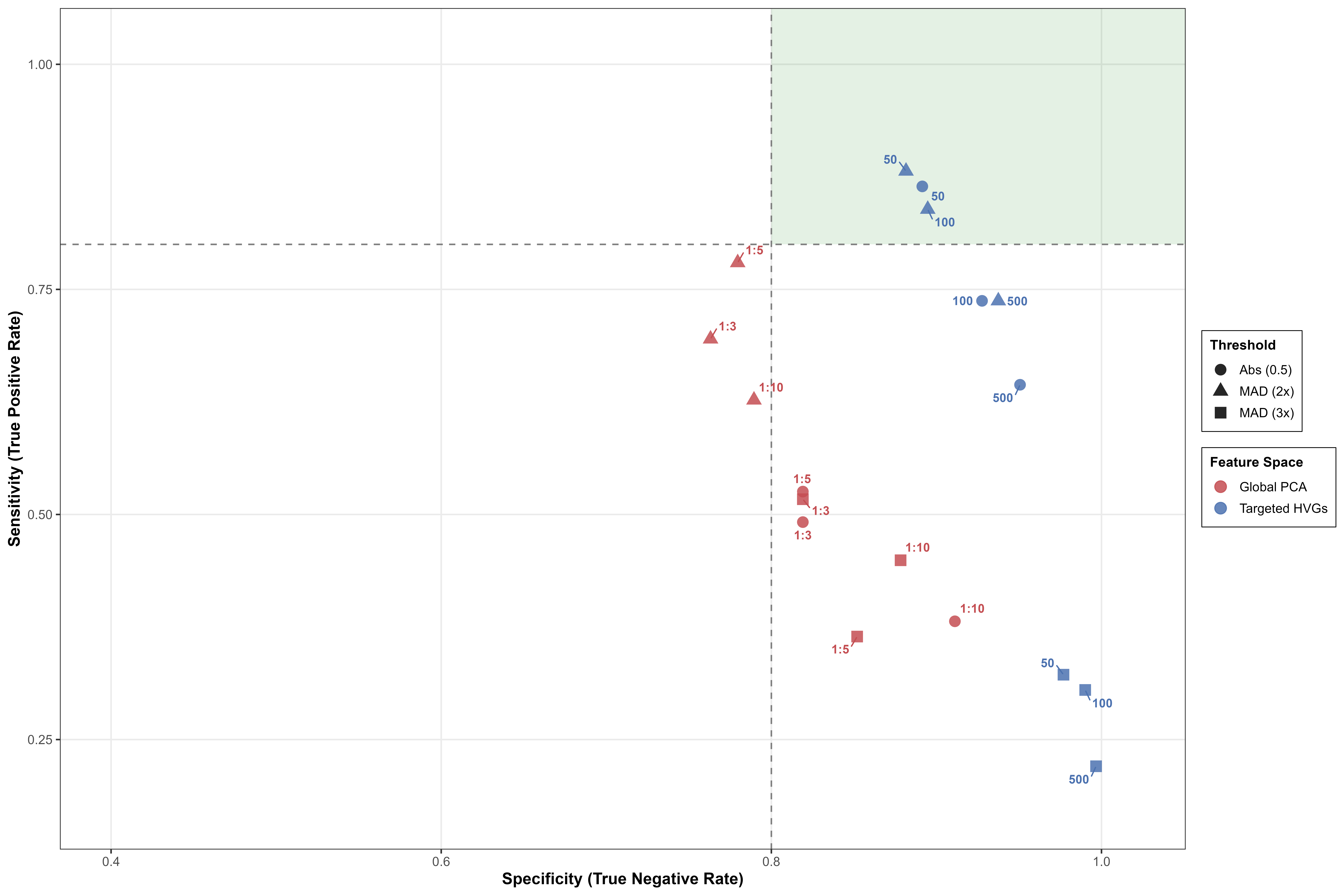
When tuning the Isolation Forest, we evaluated the use of global Principal Components (red) versus targeted Highly Variable Genes (blue) under absolute and adaptive (MAD-based) thresholds. - Finding: Calculating anomalies on a targeted subset of local HVGs (e.g., 50–500 genes) using adaptive MAD thresholds consistently yielded the best balance of Sensitivity and Specificity (upper right quadrant).
Reconstruction Error Tuning
Script: R/brain/Supplementary_Figure_6.R
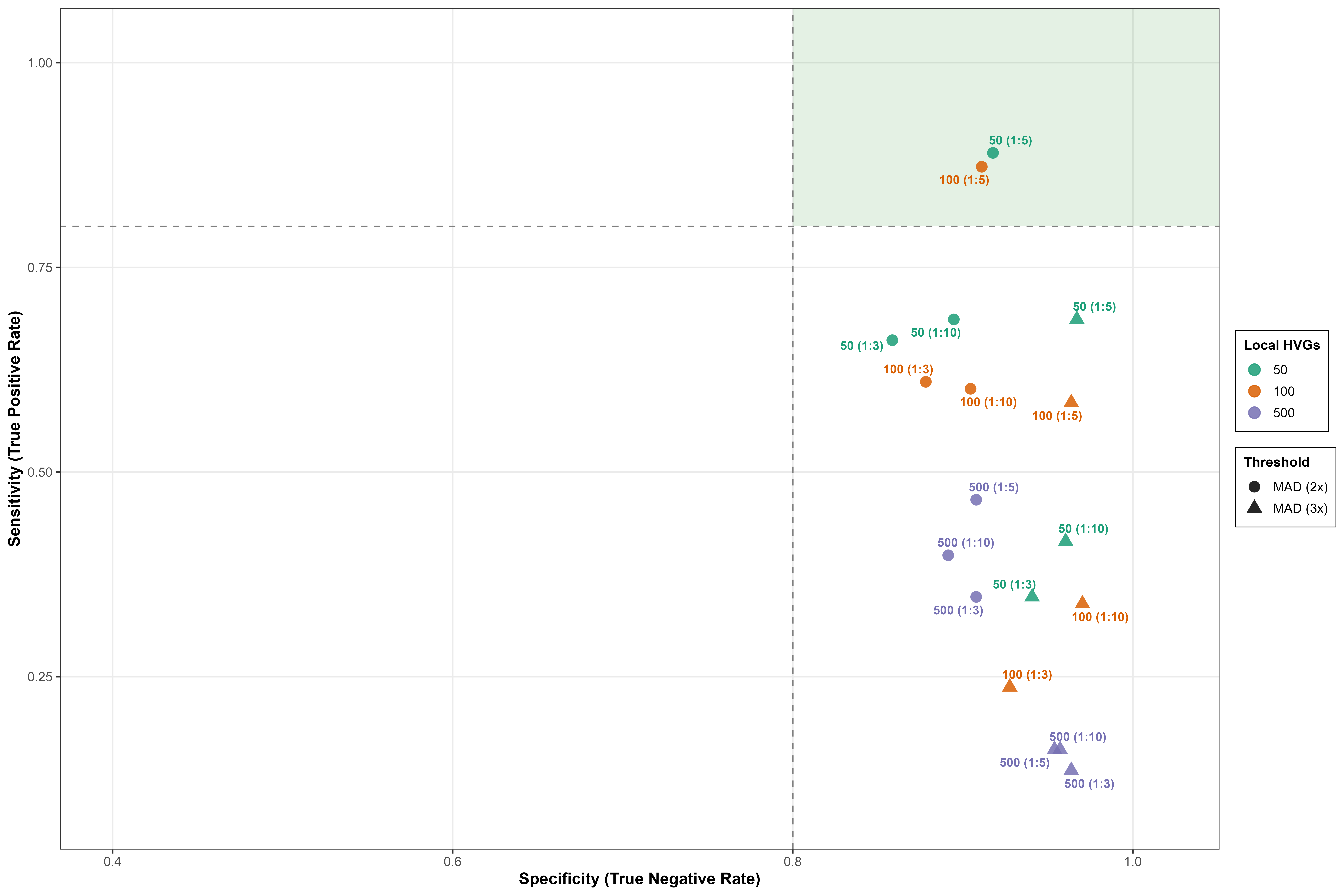
When tuning Reconstruction Error, we evaluated the interaction between the number of HVGs and the dimensionality of the PC space used for reconstruction. - Finding: Models using a compact PC subspace (PCs 1:3 or 1:5) derived from ~100 HVGs, paired with a 2x MAD threshold, consistently clustered in the high-performance “sweet spot.”
Interpretation & Recommendations
The Zeisel brain benchmarking demonstrates that scDiagnostics:
- Detects Unrepresented States: Reliably flags forced annotations across diverse biological scenarios (distinct lineages, related subtypes, rare cells).
- Resists Technical Artifacts: Maintains diagnostic power despite extreme class imbalance and moderate label noise.
- Data-Adaptive Thresholds Work: Using the reference distribution’s Median + 2x MAD provides a highly robust, dataset-agnostic threshold for flagging anomalies.
These quantitative benchmarks mirror our findings in the COVID-19 and MERFISH datasets, proving that the algorithm’s success is a feature of its statistical design, not just an artifact of a specific biological case study.