Mapping PPIs onto 3D protein structures
PDB.RmdSetup
The bioplexpy package implements functions to calculate and visualize physical interactions between chains of a PDB structure and compare with BioPlex PPIs detected in the AP-MS data.
This can be used to identify subunits of a protein complex that are close enough to physically interact. This analysis (1) maps a set of UniProt IDs, corresponding to the subunits of the complex, to a PDB structure, and (2) infers physical interactions within a structure by calculating the distance between the atoms of different chains within that structure.
Here, we demonstrate how to invoke this functionality from within R, and how to incorporate results into subsequent analysis and visualization in R.
We start by loading the required packages.
Mapping from a set of UniProt IDs to a PDB structure
We use data from the SIFTS project to map from CORUM complex subunits given as UniProt IDs to PDB structures:
url <- "ftp://ftp.ebi.ac.uk/pub/databases/msd/sifts/flatfiles/csv/uniprot_pdb.csv.gz"
dest <- basename(url)
download.file(url, destfile = dest)
df <- read.csv("uniprot_pdb.csv.gz", skip = 1)
file.remove(dest)
## [1] TRUE
head(df)## SP_PRIMARY PDB
## 1 A0A003 6kvc;6kv9
## 2 A0A009I821 7m4y;7m4x;7ryg;7m4w;7ryf;7ryh;7m4z
## 3 A0A009L7S8 7m4z;7ryh;7ryf;7m4y;7ryg;7m4w;7m4x
## 4 A0A009QSN8 6v3d;6v39;6v3b;6v3a
## 5 A0A010 6j8v;5b01;5b00;5b0i;5b0l;5b0k;5b03;5b0m;6j8w;5b02;5gww;5gwv;5b0j
## 6 A0A011 3vkb;3vka;3vk5;3vkc;3vkdTurn into a mapping:
## $A0A003
## [1] "6kvc" "6kv9"
##
## $A0A009I821
## [1] "7m4y" "7m4x" "7ryg" "7m4w" "7ryf" "7ryh" "7m4z"
##
## $A0A009L7S8
## [1] "7m4z" "7ryh" "7ryf" "7m4y" "7ryg" "7m4w" "7m4x"
##
## $A0A009QSN8
## [1] "6v3d" "6v39" "6v3b" "6v3a"
##
## $A0A010
##  [1] "6j8v" "5b01" "5b00" "5b0i" "5b0l" "5b0k" "5b03" "5b0m" "6j8w" "5b02"
## [11] "5gww" "5gwv" "5b0j"
##
## $A0A011
## [1] "3vkb" "3vka" "3vk5" "3vkc" "3vkd"
Having illustrated the basic principle underlying the mapping from a CORUM complex to a PDB structure, we now set up a python environment via reticulate that contains the bioplexpy package in order to invoke the functionality from within R, facilitating direct exchange of data and results between the BioPlex R and BioPlex Python packages:
reticulate::virtualenv_create("r-reticulate")## virtualenv: r-reticulate
reticulate::virtualenv_install("r-reticulate", "bioplexpy")## Using virtual environment 'r-reticulate' ...
reticulate::use_virtualenv("r-reticulate")
bp <- reticulate::import("bioplexpy")
In the following, we focus on the TFIIH core complex (PDB ID: 6nmi).
We first get the set of UniProt IDs corresponding to this CORUM complex ID.
corum <- bp$getCorum(complex_set = "core", organism = "Human")
unips <- bp$get_UniProts_from_CORUM(corum, 107)
unips
## [1] "P18074" "P19447" "P32780" "P50613" "P51946" "P51948" "Q13888" "Q13889"
## [9] "Q92759"and then also get the set of PDB IDs corresponding to the obtained set of UniProt IDs based on the SIFTS mapping.
pdbs <- bp$get_PDB_from_UniProts(unips)
head(pdbs)
## num_proteins deposit_date
## 7AD8 8 2020-09-14
## 6O9M 8 2019-03-14
## 6NMI 8 2019-01-10
## 5OF4 10 2017-07-10
## 7NVW 11 2021-03-16
## 7NVX 11 2021-03-16
## citation_title
## 7AD8 The TFIIH subunits p44/p62 act as a damage sensor during nucleotide excision repair.
## 6O9M Transcription preinitiation complex structure and dynamics provide insight into genetic diseases.
## 6NMI The complete structure of the human TFIIH core complex.
## 5OF4 The cryo-electron microscopy structure of human transcription factor IIH.
## 7NVW Structures of mammalian RNA polymerase II pre-initiation complexes.
## 7NVX Structures of mammalian RNA polymerase II pre-initiation complexes.
## UniProts_mapped_to_PDB num_proteins_diff_btwn_PDB_and_UniProts_input
## 7AD8 P18074, .... 1
## 6O9M P18074, .... 1
## 6NMI P18074, .... 1
## 5OF4 P18074, .... 1
## 7NVW P18074, .... 2
## 7NVX P18074, .... 2As there is often no 1:1 mapping from a set of UniProt IDs to a certain PDB structure, it is instructive to inspect the title of the PDB entry and use prior knowledge about the PDB structure for a complex of interest where available.
Here, we accordingly chose 6nmi as the PDB ID representing the TFIIH core complex.
We can use functionality from the bio3d package to get the PDB structure for the TFIIH core complex (PDB ID: 6nmi).
##
##  Call:  bio3d::read.pdb(file = pdb.file)
##
##    Total Models#: 1
##      Total Atoms#: 24379,  XYZs#: 73137  Chains#: 8  (values: A B C D E F G H)
##
##      Protein Atoms#: 23015  (residues/Calpha atoms#: 2908)
##      Nucleic acid Atoms#: 0  (residues/phosphate atoms#: 0)
##
##      Non-protein/nucleic Atoms#: 1364  (residues: 277)
##      Non-protein/nucleic resid values: [ SF4 (1), UNK (270), ZN (6) ]
##
##    Protein sequence:
##       PQEAVPSAAGKQVDESGTKVDEYGAKDYRLQMPLKDDHTSRPLWVAPDGHIFLEAFSPVY
##       KYAQDFLVAIAEPVCRPTHVHEYKLTAYSLYAAVSVGLQTSDITEYLRKLSKTGVPDGIM
##       QFIKLCTVSYGKVKLVLKHNRYFVESCHPDVIQHLLQDPVIRECRLRNSEQTVSFEVKQE
##       MIEELQKRCIHLEYPLLAEYDFRNDSVNPDINIDLKPTAVLRPYQ...<cut>...QLEM
##
## + attr: atom, xyz, seqres, helix, sheet,
##         calpha, remark, call
str(pdb)## List of 8
## $ atom :'data.frame': 24379 obs. of 16 variables:
## ..$ type : chr [1:24379] "ATOM" "ATOM" "ATOM" "ATOM" ...
## ..$ eleno : int [1:24379] 1 2 3 4 5 6 7 8 9 10 ...
## ..$ elety : chr [1:24379] "N" "CA" "C" "O" ...
## ..$ alt : chr [1:24379] NA NA NA NA ...
## ..$ resid : chr [1:24379] "PRO" "PRO" "PRO" "PRO" ...
## ..$ chain : chr [1:24379] "A" "A" "A" "A" ...
## ..$ resno : int [1:24379] 34 34 34 34 34 34 34 35 35 35 ...
## ..$ insert: chr [1:24379] NA NA NA NA ...
## ..$ x : num [1:24379] 177 177 175 175 177 ...
## ..$ y : num [1:24379] 185 185 185 186 186 ...
## ..$ z : num [1:24379] 131 133 133 133 133 ...
## ..$ o : num [1:24379] 1 1 1 1 1 1 1 1 1 1 ...
## ..$ b : num [1:24379] 60.6 60.6 60.6 60.6 60.6 ...
## ..$ segid : chr [1:24379] NA NA NA NA ...
## ..$ elesy : chr [1:24379] "N" "C" "C" "O" ...
## ..$ charge: chr [1:24379] NA NA NA NA ...
## $ xyz : 'xyz' num [1, 1:73137] 177 185 131 177 185 ...
## $ seqres: Named chr [1:3477] "PRO" "GLN" "GLU" "ALA" ...
## ..- attr(*, "names")= chr [1:3477] "A" "A" "A" "A" ...
## $ helix :List of 4
## ..$ start: Named num [1:128] 37 92 119 132 149 181 191 249 273 276 ...
## .. ..- attr(*, "names")= chr [1:128] "" "" "" "" ...
## ..$ end : Named num [1:128] 42 104 130 142 161 190 198 262 275 287 ...
## .. ..- attr(*, "names")= chr [1:128] "" "" "" "" ...
## ..$ chain: chr [1:128] "A" "A" "A" "A" ...
## ..$ type : chr [1:128] "1" "1" "1" "1" ...
## $ sheet :List of 4
## ..$ start: Named num [1:80] 59 333 342 314 307 76 83 113 105 268 ...
## .. ..- attr(*, "names")= chr [1:80] "" "" "" "" ...
## ..$ end : Named num [1:80] 60 337 345 317 310 78 87 117 108 272 ...
## .. ..- attr(*, "names")= chr [1:80] "" "" "" "" ...
## ..$ chain: chr [1:80] "A" "D" "D" "D" ...
## ..$ sense: chr [1:80] "0" "1" "-1" "-1" ...
## $ calpha: logi [1:24379] FALSE TRUE FALSE FALSE FALSE FALSE ...
## $ remark:List of 1
## ..$ biomat:List of 4
## .. ..$ num : int 1
## .. ..$ chain :List of 1
## .. .. ..$ : chr [1:8] "A" "B" "C" "D" ...
## .. ..$ mat :List of 1
## .. .. ..$ :List of 1
## .. .. .. ..$ A B C D E F G H: num [1:3, 1:4] 1 0 0 0 1 0 0 0 1 0 ...
## .. ..$ method: chr "AUTHOR"
## $ call : language bio3d::read.pdb(file = pdb.file)
## - attr(*, "class")= chr [1:2] "pdb" "sse"Provide a different color for each chain:
chains <- unlist(pdb$remark$biomat$chain)
chains
## [1] "A" "B" "C" "D" "E" "F" "G" "H"
nr.chains <- length(chains)
chain.colors <- RColorBrewer::brewer.pal(8, "Set1")
chain.colors <- tolower(chain.colors)
And visualize the structure using functionality from the r3dmol package:
# Set up the initial viewer
viewer <- r3dmol(
  id = "",
  elementId = "demo"
) %>%
  # Add model to scene
  m_add_model(data = m_bio3d(pdb), format = "pdb") %>%
  # Zoom to encompass the whole scene
  m_zoom_to() %>%
  # Set style of structures
  m_set_style(style = m_style_cartoon(color = "#00cc96"))
for(i in seq_len(nr.chains))
  viewer <- m_set_style(viewer,
    sel = m_sel(chain = LETTERS[i]),
    style = m_style_cartoon(color = chain.colors[i])
  )
viewer %>% m_rotate(angle = 90, axis = "y") %>% m_spin()
Identify interacting chains within a protein structure
We infer physical interactions within a structure by calculating the distance between the atoms of different chains within that structure. The coordinates of each atom can be obtained directly from the PDB file.
##   type chain       x       y       z
## 1 ATOM     A 177.229 185.012 131.416
## 2 ATOM     A 176.734 185.041 132.796
## 3 ATOM     A 175.216 185.196 132.898
## 4 ATOM     A 174.716 186.287 133.174
## 5 ATOM     A 177.452 186.253 133.398
## 6 ATOM     A 177.785 187.117 132.235
If the minimum distance between atoms of two chains is below a given threshold (default: 6 angstrom), these proteins are defined to interact directly; all other pairs of proteins that occurred in the same structure are assumed to interact indirectly.
ia.chains <- bp$get_interacting_chains_from_PDB('6NMI', '.', 6)
ia.chains
## [[1]]
## [1] "A" "B"
##
## [[2]]
## [1] "A" "D"
##
## [[3]]
## [1] "A" "E"
##
## [[4]]
## [1] "A" "G"
##
## [[5]]
## [1] "A" "H"
##
## [[6]]
## [1] "B" "C"
##
## [[7]]
## [1] "B" "E"
##
## [[8]]
## [1] "B" "H"
##
## [[9]]
## [1] "C" "D"
##
## [[10]]
## [1] "C" "E"
##
## [[11]]
## [1] "C" "F"
##
## [[12]]
## [1] "D" "F"
##
## [[13]]
## [1] "D" "G"
##
## [[14]]
## [1] "E" "F"For example, this demonstrates that chain A (red) and chain B (blue) are in close proximity, and that both chains are also close to chain H (pink), as evident from the structure view above.
Once we have obtained the list of interacting chains, we map each chain to a UNIPROT ID, again based on data from the SIFTS project.
chain2unip <- bp$list_uniprot_pdb_mappings('6NMI')
chain2unip
## $B
## [1] "P18074"
##
## $A
## [1] "P19447"
##
## $E
## [1] "Q13888"
##
## $D
## [1] "Q92759"
##
## $F
## [1] "Q13889"
##
## $H
## [1] "P51948"
##
## $C
## [1] "P32780"
##
## $G
## [1] "Q6ZYL4"This mapping now allows us to produce a list of interacting chains using their corresponding UNIPROT ID.
chain2unip <- unlist(chain2unip)
ia.unips <- lapply(ia.chains, function(x) unname(chain2unip[x]))
ia.unips
## [[1]]
## [1] "P19447" "P18074"
##
## [[2]]
## [1] "P19447" "Q92759"
##
## [[3]]
## [1] "P19447" "Q13888"
##
## [[4]]
## [1] "P19447" "Q6ZYL4"
##
## [[5]]
## [1] "P19447" "P51948"
##
## [[6]]
## [1] "P18074" "P32780"
##
## [[7]]
## [1] "P18074" "Q13888"
##
## [[8]]
## [1] "P18074" "P51948"
##
## [[9]]
## [1] "P32780" "Q92759"
##
## [[10]]
## [1] "P32780" "Q13888"
##
## [[11]]
## [1] "P32780" "Q13889"
##
## [[12]]
## [1] "Q92759" "Q13889"
##
## [[13]]
## [1] "Q92759" "Q6ZYL4"
##
## [[14]]
## [1] "Q13888" "Q13889"We reshape this list to a data.frame:
ia1 <- vapply(ia.unips, `[`, character(1), x = 1)
ia2 <- vapply(ia.unips, `[`, character(1), x = 2)
ia.df <- data.frame(CHAIN1 = ia1, CHAIN2 = ia2)
ia.df
## CHAIN1 CHAIN2
## 1 P19447 P18074
## 2 P19447 Q92759
## 3 P19447 Q13888
## 4 P19447 Q6ZYL4
## 5 P19447 P51948
## 6 P18074 P32780
## 7 P18074 Q13888
## 8 P18074 P51948
## 9 P32780 Q92759
## 10 P32780 Q13888
## 11 P32780 Q13889
## 12 Q92759 Q13889
## 13 Q92759 Q6ZYL4
## 14 Q13888 Q13889Identify interactions that are also detected in the BioPlex network
Having inferred physical interactions between subunits of the TFIIH core complex, we can now investigate which of these interactions have been detected in the BioPlex PPI data.
We therefore first look at all possible edges with the TFIIH core complex, and subsequently contrast that with edges detected in the BioPlex network and the inferred direct interactions from the PDB data.
corum.df <- BioPlex::getCorum("core")## Using cached version from 2023-01-14 23:43:08
corum.glist <- BioPlex::corum2graphlist(corum.df)
tfiih.gr <- corum.glist[["CORUM107_TFIIH_transcription_factor_complex"]]
tfiih.gr
## A graphNEL graph with undirected edges
## Number of Nodes = 9
## Number of Edges = 36
BioPlexAnalysis::plotGraph(tfiih.gr, edge.mode = "undirected",
                           edge.color = "grey", layout = "circle")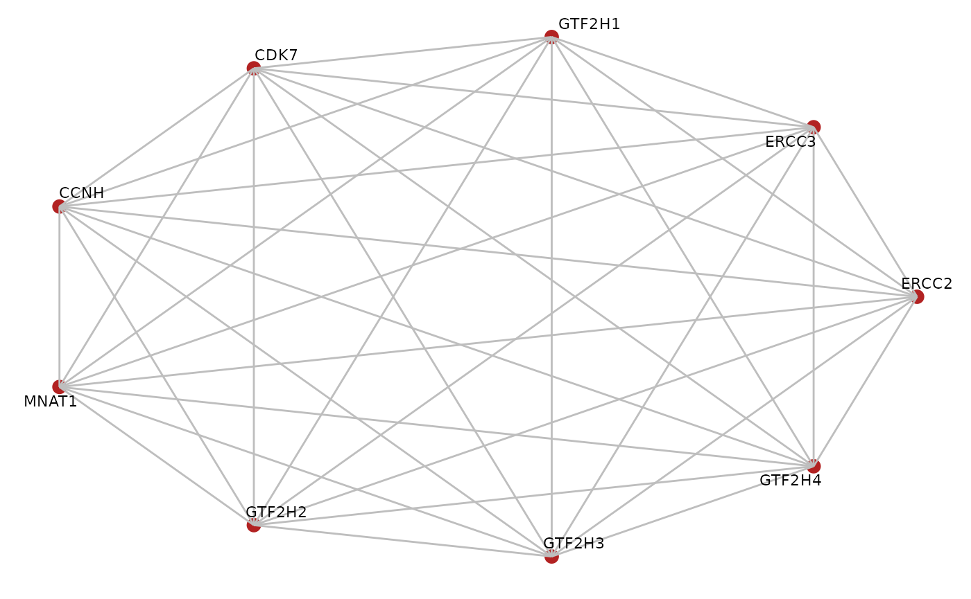
Now we obtain the latest version of the BioPlex network for the 293T cell line,
bp.293t <- BioPlex::getBioPlex(cell.line = "293T", version = "3.0")## Using cached version from 2023-01-14 23:15:28
bp.gr <- BioPlex::bioplex2graph(bp.293t)and subset the bioplex network to edges between subunits of the TFIIH core complex.
bp.tfiih <- graph::subGraph(unips, bp.gr)
bp.tfiih.edges <- graph::edges(bp.tfiih)
bp.tfiih.edges <- stack(bp.tfiih.edges)
bp.tfiih.edges$ind <- as.character(bp.tfiih.edges$ind)
Let’s visually inspect the edges between subunits of the complex that have been detected in the BioPlex network.
graph::edgeDataDefaults(tfiih.gr, "type") <- "not detected"
graph::edgeData(tfiih.gr,
                bp.tfiih.edges$ind,
                bp.tfiih.edges$values,
                "type") <- "detected"
BioPlexAnalysis::plotGraph(tfiih.gr,
                           edge.mode = "undirected",
                           edge.color = "grey",
                           layout = "circle",
                           edge.data = "type")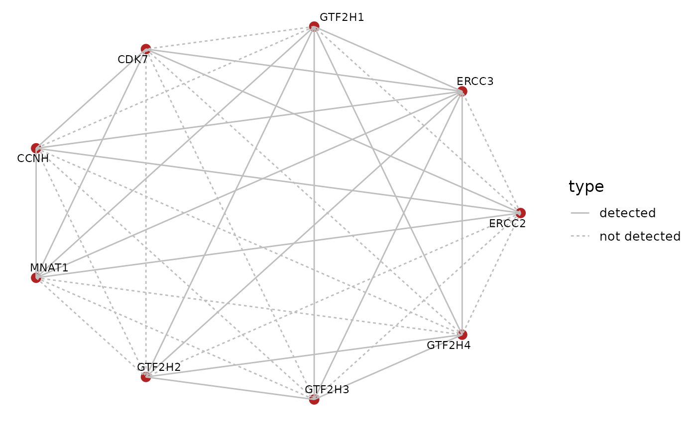
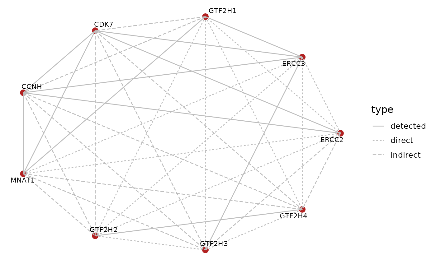
We can contrast this with the edges that we have inferred to directly interact with each other from proximity of the chains within the PDB structure.
ia.df <- subset(ia.df, CHAIN2 != "Q6ZYL4")
graph::edgeDataDefaults(tfiih.gr, "type") <- "indirect"
graph::edgeData(tfiih.gr,
                ia.df$CHAIN1,
                ia.df$CHAIN2,
                "type") <- "direct"
BioPlexAnalysis::plotGraph(tfiih.gr,
                           edge.mode = "undirected",
                           edge.color = "grey",
                           layout = "circle",
                           edge.data = "type")