Introduction to Bioconductor and the SingleCellExperiment class
Last updated on 2024-11-11 | Edit this page
Estimated time: 30 minutes
Overview
Questions
- What is Bioconductor?
- How is single-cell data stored in the Bioconductor ecosystem?
- What is a
SingleCellExperimentobject?
Objectives
- Install and update Bioconductor packages.
- Load data generated with common single-cell technologies as
SingleCellExperimentobjects. - Inspect and manipulate
SingleCellExperimentobjects.
Bioconductor
Overview
Within the R ecosystem, the Bioconductor project provides tools for the analysis and comprehension of high-throughput genomics data. The scope of the project covers microarray data, various forms of sequencing (RNA-seq, ChIP-seq, bisulfite, genotyping, etc.), proteomics, flow cytometry and more. One of Bioconductor’s main selling points is the use of common data structures to promote interoperability between packages, allowing code written by different people (from different organizations, in different countries) to work together seamlessly in complex analyses.
Installing Bioconductor Packages
The default repository for R packages is the Comprehensive R Archive Network (CRAN), which is home to over 13,000 different R packages. We can easily install packages from CRAN - say, the popular ggplot2 package for data visualization - by opening up R and typing in:
R
install.packages("ggplot2")
In our case, however, we want to install Bioconductor packages. These packages are located in a separate repository hosted by Bioconductor, so we first install the BiocManager package to easily connect to the Bioconductor servers.
R
install.packages("BiocManager")
After that, we can use BiocManager’s
install() function to install any package from
Bioconductor. For example, the code chunk below uses this approach to
install the SingleCellExperiment
package.
R
BiocManager::install("SingleCellExperiment")
Should we forget, the same instructions are present on the landing
page of any Bioconductor package. For example, looking at the scater
package page on Bioconductor, we can see the following copy-pasteable
instructions:
R
if (!requireNamespace("BiocManager", quietly = TRUE))
    install.packages("BiocManager")

BiocManager::install("scater")
Packages only need to be installed once, and then they are available for all subsequent uses of a particular R installation. There is no need to repeat the installation every time we start R.
Finding relevant packages
To find relevant Bioconductor packages, one useful resource is the BiocViews page. This provides a hierarchically organized view of annotations associated with each Bioconductor package. For example, under the “Software” label, we might be interested in a particular “Technology” such as… say, “SingleCell”. This gives us a listing of all Bioconductor packages that might be useful for our single-cell data analyses. CRAN uses the similar concept of “Task views”, though this is understandably more general than genomics. For example, the Cluster task view page lists an assortment of packages that are relevant to cluster analyses.
Staying up to date
Updating all R/Bioconductor packages is as simple as running
BiocManager::install() without any arguments. This will
check for more recent versions of each package (within a Bioconductor
release) and prompt the user to update if any are available.
R
BiocManager::install()
This might take some time if many packages need to be updated, but is typically recommended to avoid issues resulting from outdated package versions.
The SingleCellExperiment class
Setup
We start by loading some libraries we’ll be using:
R
library(SingleCellExperiment)
library(MouseGastrulationData)
It is normal to see lot of startup messages when loading these packages.
Motivation and overview
One of the main strengths of the Bioconductor project lies in the use of a common data infrastructure that powers interoperability across packages.
Users should be able to analyze their data using functions from
different Bioconductor packages without the need to convert between
formats. To this end, the SingleCellExperiment class (from
the SingleCellExperiment package) serves as the common currency
for data exchange across 70+ single-cell-related Bioconductor
packages.
This class implements a data structure that stores all aspects of our single-cell data - gene-by-cell expression data, cell-wise metadata, and gene-wise annotation - and lets us manipulate them in an organized manner.
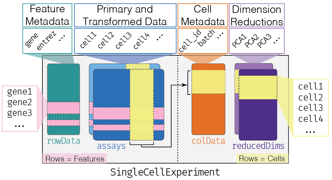
The complexity of the SingleCellExperiment container
might be a little bit intimidating in the beginning. One might be
tempted to use a simpler approach by just keeping all of these
components in separate objects, e.g. a matrix of counts, a
data.frame of sample metadata, a data.frame of
gene annotations, and so on.
There are two main disadvantages to this “from-scratch” approach:
- It requires a substantial amount of manual bookkeeping to keep the different data components in sync. If you performed a QC step that removed dead cells from the count matrix, you also had to remember to remove that same set of cells from the cell-wise metadata. Did you filtered out genes that did not display sufficient expression levels to be retained for further analysis? Then you would need to make sure to not forget to filter the gene metadata table too.
- All the downstream steps had to be “from scratch” as well. All the data munging, analysis, and visualization code had to be customized to the idiosyncrasies of a given input set.
Let’s look at an example dataset. WTChimeraData comes
from a study on mouse development Pijuan-Sala et
al.. The study profiles the effect of a transcription factor TAL1
and its influence on mouse development. Because mutations in this gene
can cause severe developmental issues, Tal1-/- cells (positive for
tdTomato, a fluorescent protein) were injected into wild-type
blastocysts (tdTomato-), forming chimeric embryos.
We can assign one sample to a SingleCellExperiment
object named sce like so:
R
sce <- WTChimeraData(samples = 5)

sce
OUTPUT
class: SingleCellExperiment
dim: 29453 2411
metadata(0):
assays(1): counts
rownames(29453): ENSMUSG00000051951 ENSMUSG00000089699 ...
  ENSMUSG00000095742 tomato-td
rowData names(2): ENSEMBL SYMBOL
colnames(2411): cell_9769 cell_9770 ... cell_12178 cell_12179
colData names(11): cell barcode ... doub.density sizeFactor
reducedDimNames(2): pca.corrected.E7.5 pca.corrected.E8.5
mainExpName: NULL
altExpNames(0):
We can think of this (and other) class as a container, that contains several different pieces of data in so-called slots. SingleCellExperiment objects come with dedicated methods for getting and setting the data in their slots.
Depending on the object, slots can contain different types of data (e.g., numeric matrices, lists, etc.). Here we’ll review the main slots of the SingleCellExperiment class as well as their getter/setter methods.
Challenge
Get the data for a different sample from WTChimeraData
(other than the fifth one).
Here we obtain the sixth sample and assign it to
sce6:
R
sce6 <- WTChimeraData(samples = 6)

sce6
assays
This is arguably the most fundamental part of the object that
contains the count matrix, and potentially other matrices with
transformed data. We can access the list of matrices with the
assays function and individual matrices with the
assay function. If one of these matrices is called
“counts”, we can use the special counts getter (likewise
for logcounts).
R
names(assays(sce))
OUTPUT
[1] "counts"R
counts(sce)[1:3, 1:3]
OUTPUT
3 x 3 sparse Matrix of class "dgCMatrix"
                   cell_9769 cell_9770 cell_9771
ENSMUSG00000051951         .         .         .
ENSMUSG00000089699         .         .         .
ENSMUSG00000102343         .         .         .
You will notice that in this case we have a sparse matrix of class
dgTMatrix inside the object. More generally, any
“matrix-like” object can be used, e.g., dense matrices or HDF5-backed
matrices (as we will explore later in the Working
with large data episode).
colData and rowData
Conceptually, these are two data frames that annotate the columns and the rows of your assay, respectively.
One can interact with them as usual, e.g., by extracting columns or adding additional variables as columns.
R
colData(sce)[1:3, 1:4]
OUTPUT
DataFrame with 3 rows and 4 columns
                 cell          barcode    sample       stage
          <character>      <character> <integer> <character>
cell_9769   cell_9769 AAACCTGAGACTGTAA         5        E8.5
cell_9770   cell_9770 AAACCTGAGATGCCTT         5        E8.5
cell_9771   cell_9771 AAACCTGAGCAGCCTC         5        E8.5
R
rowData(sce)[1:3, 1:2]
OUTPUT
DataFrame with 3 rows and 2 columns
                              ENSEMBL      SYMBOL
                          <character> <character>
ENSMUSG00000051951 ENSMUSG00000051951        Xkr4
ENSMUSG00000089699 ENSMUSG00000089699      Gm1992
ENSMUSG00000102343 ENSMUSG00000102343     Gm37381
You can access columns of the colData with the $
accessor to quickly add cell-wise metadata to the
colData.
R
sce$my_sum <- colSums(counts(sce))

colData(sce)[1:3,]
OUTPUT
DataFrame with 3 rows and 12 columns
                 cell          barcode    sample       stage    tomato
          <character>      <character> <integer> <character> <logical>
cell_9769   cell_9769 AAACCTGAGACTGTAA         5        E8.5      TRUE
cell_9770   cell_9770 AAACCTGAGATGCCTT         5        E8.5      TRUE
cell_9771   cell_9771 AAACCTGAGCAGCCTC         5        E8.5      TRUE
               pool stage.mapped celltype.mapped closest.cell doub.density
          <integer>  <character>     <character>  <character>    <numeric>
cell_9769         3        E8.25      Mesenchyme   cell_24159   0.02985045
cell_9770         3         E8.5     Endothelium   cell_96660   0.00172753
cell_9771         3         E8.5       Allantois  cell_134982   0.01338013
          sizeFactor    my_sum
           <numeric> <numeric>
cell_9769    1.41243     27577
cell_9770    1.22757     29309
cell_9771    1.15439     28795
Challenge
Add a column of gene-wise metadata to the rowData.
Here, we add a column named conservation that could
represent an evolutionary conservation score.
R
rowData(sce)$conservation <- rnorm(nrow(sce))
This is just an example for demonstration purposes, but in practice
it is convenient and simplifies data management to store any sort of
gene-wise information in the columns of the rowData.
The reducedDims
Everything that we have described so far (except for the
counts getter) is part of the
SummarizedExperiment class that
SingleCellExperiment extends. You can find a complete
lesson on the SummarizedExperiment class in Introduction
to data analysis with R and Bioconductor course.
One peculiarity of SingleCellExperiment is its ability
to store reduced dimension matrices within the object. These may include
PCA, t-SNE, UMAP, etc.
R
reducedDims(sce)
OUTPUT
List of length 2
names(2): pca.corrected.E7.5 pca.corrected.E8.5
As for the other slots, we have the usual setter/getter, but it is somewhat rare to interact directly with these functions.
It is more common for other functions to store this
information in the object, e.g., the runPCA function from
the scater package.
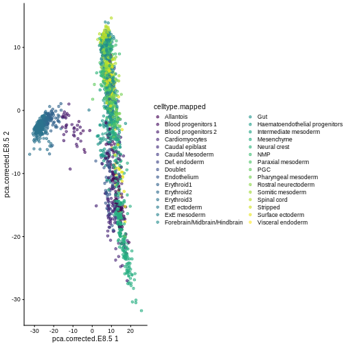
Here, we use scater’s plotReducedDim
function as an example of how to extract this information
indirectly from the objects. Note that one could obtain the
same results (somewhat less efficiently) by extracting the corresponding
reducedDim matrix and ggplot.
R
library(scater)

plotReducedDim(sce, "pca.corrected.E8.5", colour_by = "celltype.mapped")
Exercise 1
Create a SingleCellExperiment object “from scratch”.
That means: start from a matrix (either randomly generated
or with some fake data in it) and add one or more columns as
colData.
The SingleCellExperiment constructor function can be
used to create a new SingleCellExperiment object.
R
mat <- matrix(runif(30), ncol = 5)

my_sce <- SingleCellExperiment(assays = list(logcounts = mat))

my_sce$my_col_info = runif(5)

my_sce
OUTPUT
class: SingleCellExperiment
dim: 6 5
metadata(0):
assays(1): logcounts
rownames: NULL
rowData names(0):
colnames: NULL
colData names(1): my_col_info
reducedDimNames(0):
mainExpName: NULL
altExpNames(0):
Exercise 2
Combine two SingleCellExperiment objects. The
MouseGastrulationData package contains several datasets.
Download sample 6 of the chimera experiment. Use the cbind
function to combine the new data with the sce object
created before.
R
sce  <- WTChimeraData(samples = 5)

sce6 <- WTChimeraData(samples = 6)

combined_sce <- cbind(sce, sce6)

combined_sce
OUTPUT
class: SingleCellExperiment
dim: 29453 3458
metadata(0):
assays(1): counts
rownames(29453): ENSMUSG00000051951 ENSMUSG00000089699 ...
  ENSMUSG00000095742 tomato-td
rowData names(2): ENSEMBL SYMBOL
colnames(3458): cell_9769 cell_9770 ... cell_13225 cell_13226
colData names(11): cell barcode ... doub.density sizeFactor
reducedDimNames(2): pca.corrected.E7.5 pca.corrected.E8.5
mainExpName: NULL
altExpNames(0):
Further Reading
- OSCA book, Introduction
Key Points
- The Bioconductor project provides open-source software packages for the comprehension of high-throughput biological data.
- A
SingleCellExperimentobject is an extension of theSummarizedExperimentobject. -
SingleCellExperimentobjects contain specialized data fields for storing data unique to single-cell analyses, such as thereducedDimsfield.
References
- Pijuan-Sala B, Griffiths JA, Guibentif C et al. (2019). A single-cell molecular map of mouse gastrulation and early organogenesis. Nature 566, 7745:490-495.
Session Info
R
sessionInfo()
OUTPUT
R version 4.4.1 (2024-06-14)
Platform: x86_64-pc-linux-gnu
Running under: Ubuntu 22.04.5 LTS

Matrix products: default
BLAS:   /usr/lib/x86_64-linux-gnu/blas/libblas.so.3.10.0
LAPACK: /usr/lib/x86_64-linux-gnu/lapack/liblapack.so.3.10.0

locale:
 [1] LC_CTYPE=C.UTF-8       LC_NUMERIC=C           LC_TIME=C.UTF-8
 [4] LC_COLLATE=C.UTF-8     LC_MONETARY=C.UTF-8    LC_MESSAGES=C.UTF-8
 [7] LC_PAPER=C.UTF-8       LC_NAME=C              LC_ADDRESS=C
[10] LC_TELEPHONE=C         LC_MEASUREMENT=C.UTF-8 LC_IDENTIFICATION=C

time zone: UTC
tzcode source: system (glibc)

attached base packages:
[1] stats4    stats     graphics  grDevices utils     datasets  methods
[8] base

other attached packages:
 [1] scater_1.32.0                ggplot2_3.5.1
 [3] scuttle_1.14.0               MouseGastrulationData_1.18.0
 [5] SpatialExperiment_1.14.0     SingleCellExperiment_1.26.0
 [7] SummarizedExperiment_1.34.0  Biobase_2.64.0
 [9] GenomicRanges_1.56.0         GenomeInfoDb_1.40.1
[11] IRanges_2.38.0               S4Vectors_0.42.0
[13] BiocGenerics_0.50.0          MatrixGenerics_1.16.0
[15] matrixStats_1.3.0            BiocStyle_2.32.0

loaded via a namespace (and not attached):
 [1] DBI_1.2.3                 formatR_1.14
 [3] gridExtra_2.3             rlang_1.1.3
 [5] magrittr_2.0.3            compiler_4.4.1
 [7] RSQLite_2.3.7             DelayedMatrixStats_1.26.0
 [9] png_0.1-8                 vctrs_0.6.5
[11] pkgconfig_2.0.3           crayon_1.5.2
[13] fastmap_1.2.0             dbplyr_2.5.0
[15] magick_2.8.3              XVector_0.44.0
[17] labeling_0.4.3            utf8_1.2.4
[19] rmarkdown_2.27            UCSC.utils_1.0.0
[21] ggbeeswarm_0.7.2          purrr_1.0.2
[23] bit_4.0.5                 xfun_0.44
[25] zlibbioc_1.50.0           cachem_1.1.0
[27] beachmat_2.20.0           jsonlite_1.8.8
[29] blob_1.2.4                highr_0.11
[31] DelayedArray_0.30.1       BiocParallel_1.38.0
[33] irlba_2.3.5.1             parallel_4.4.1
[35] R6_2.5.1                  Rcpp_1.0.12
[37] knitr_1.47                Matrix_1.7-0
[39] tidyselect_1.2.1          viridis_0.6.5
[41] abind_1.4-5               yaml_2.3.8
[43] codetools_0.2-20          curl_5.2.1
[45] lattice_0.22-6            tibble_3.2.1
[47] withr_3.0.0               KEGGREST_1.44.0
[49] BumpyMatrix_1.12.0        evaluate_0.23
[51] BiocFileCache_2.12.0      ExperimentHub_2.12.0
[53] Biostrings_2.72.1         pillar_1.9.0
[55] BiocManager_1.30.23       filelock_1.0.3
[57] renv_1.0.11               generics_0.1.3
[59] BiocVersion_3.19.1        sparseMatrixStats_1.16.0
[61] munsell_0.5.1             scales_1.3.0
[63] glue_1.7.0                tools_4.4.1
[65] AnnotationHub_3.12.0      BiocNeighbors_1.22.0
[67] ScaledMatrix_1.12.0       cowplot_1.1.3
[69] grid_4.4.1                AnnotationDbi_1.66.0
[71] colorspace_2.1-0          GenomeInfoDbData_1.2.12
[73] beeswarm_0.4.0            BiocSingular_1.20.0
[75] vipor_0.4.7               cli_3.6.2
[77] rsvd_1.0.5                rappdirs_0.3.3
[79] fansi_1.0.6               viridisLite_0.4.2
[81] S4Arrays_1.4.1            dplyr_1.1.4
[83] gtable_0.3.5              digest_0.6.35
[85] ggrepel_0.9.5             SparseArray_1.4.8
[87] farver_2.1.2              rjson_0.2.21
[89] memoise_2.0.1             htmltools_0.5.8.1
[91] lifecycle_1.0.4           httr_1.4.7
[93] mime_0.12                 bit64_4.0.5