Calculate Cell Similarity Using PCA Loadings
Source:R/calculateCellSimilarityPCA.R, R/plot.calculateCellSimilarityPCAObject.R
calculateCellSimilarityPCA.RdThis function calculates the cosine similarity between cells based on the principal components (PCs) obtained from PCA (Principal Component Analysis) loadings.
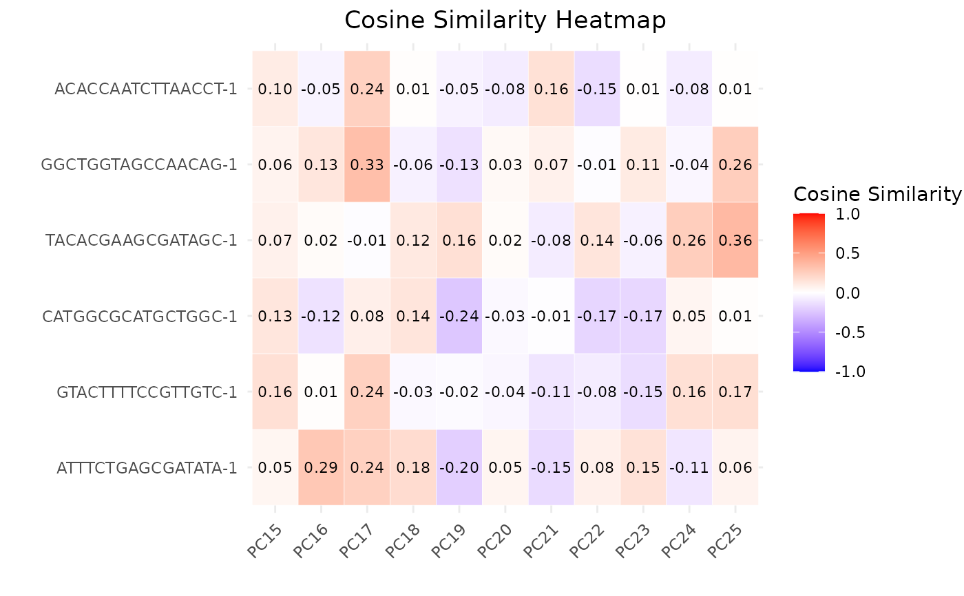
The S3 plot method creates a heatmap plot to visualize the cosine similarities between cells and principal components (PCs).
Usage
calculateCellSimilarityPCA(
  sce_object,
  cell_names,
  pc_subset = 1:5,
  n_top_vars = 50,
  assay_name = "logcounts"
)

# S3 method for class 'calculateCellSimilarityPCAObject'
plot(x, pc_subset = 1:5, ...)
Arguments
- sce_object
A
SingleCellExperimentobject containing expression data.- cell_names
A character vector specifying the cell names for which to compute the similarity.
- pc_subset
A numeric vector specifying the subset of principal components to include in the plot. Default is 1:5.
- n_top_vars
An integer indicating the number of top loading variables to consider for each PC. Default is 50.
- assay_name
Name of the assay on which to perform computations. Default is "logcounts".
- x
An object of class `calculateCellSimilarityPCA` containing a dataframe of cosine similarity values between cells and PCs.
- ...
Additional arguments passed to the plotting function.
Value
A data frame containing cosine similarity values between cells for each selected principal component.
The S3 plot method returns a ggplot object representing the cosine similarity heatmap.
Details
This function calculates the cosine similarity between cells based on the loadings of the selected
principal components obtained from PCA. It extracts the rotation matrix from the PCA results of the
SingleCellExperiment object and identifies the high-loading variables for each selected PC.
Then, it computes the cosine similarity between cells using the high-loading variables for each PC.
The S3 plot method reshapes the input data frame to create a long format suitable for plotting as a heatmap. It then creates a heatmap plot using ggplot2, where the x-axis represents the PCs, the y-axis represents the cells, and the color intensity represents the cosine similarity values.
Author
Anthony Christidis, anthony-alexander_christidis@hms.harvard.edu
Examples
# Load data
data("reference_data")
data("query_data")

# Store PCA anomaly data and plots
anomaly_output <- detectAnomaly(reference_data = reference_data,
                                query_data = query_data,
                                ref_cell_type_col = "expert_annotation",
                                query_cell_type_col = "SingleR_annotation",
                                pc_subset = 1:10,
                                n_tree = 500,
                                anomaly_threshold = 0.5)
top6_anomalies <- names(sort(anomaly_output$Combined$reference_anomaly_scores,
                             decreasing = TRUE)[1:6])

# Compute cosine similarity between anomalies and top PCs
cosine_similarities <- calculateCellSimilarityPCA(reference_data,
                                                  cell_names = top6_anomalies,
                                                  pc_subset = 1:25,
                                                  n_top_vars = 50)
cosine_similarities
#>                           PC1         PC2        PC3         PC4        PC5
#> ACACCAATCTTAACCT-1 -0.4339110  0.09963651  0.3110854 -0.08549224 -0.4661250
#> GGCTGGTAGCCAACAG-1 -0.1681258  0.11032005 -0.3459655  0.12366785 -0.4343250
#> CATGGCGCATGCTGGC-1 -0.4543269 -0.13915218 -0.1297861  0.42427682 -0.4812924
#> TACACGAAGCGATAGC-1  0.1963692  0.35033672  0.3592792  0.26904778 -0.3701442
#> GTACTTTTCCGTTGTC-1 -0.1021777  0.31110592  0.2177546  0.18410164  0.1572341
#> ATTTCTGAGCGATATA-1 -0.1511318  0.35997557 -0.3094156  0.25524359 -0.4173836
#>                            PC6         PC7         PC8         PC9       PC10
#> ACACCAATCTTAACCT-1  0.08965511 -0.28471345 -0.03848145 -0.02509098  0.1984070
#> GGCTGGTAGCCAACAG-1 -0.44398087  0.44270822  0.20765271  0.32789078 -0.2897046
#> CATGGCGCATGCTGGC-1 -0.03646835 -0.27812421 -0.06673205  0.03553433  0.4146546
#> TACACGAAGCGATAGC-1 -0.04491305 -0.13313434 -0.22034812 -0.03196268  0.3863550
#> GTACTTTTCCGTTGTC-1  0.34378011 -0.04846996  0.15205252 -0.06588815  0.1151667
#> ATTTCTGAGCGATATA-1 -0.43443550  0.50350174  0.18993881  0.23150141 -0.2185454
#>                          PC11        PC12          PC13         PC14       PC15
#> ACACCAATCTTAACCT-1 -0.4923395  0.17826466 -0.3202226875  0.312132975 0.09964316
#> GGCTGGTAGCCAACAG-1 -0.2087768  0.06268242 -0.0026756314 -0.030647911 0.06246700
#> CATGGCGCATGCTGGC-1 -0.2411911  0.22173854 -0.3039888814  0.049363044 0.12935983
#> TACACGAAGCGATAGC-1 -0.5287059  0.18751592 -0.4558131990  0.108185967 0.07114757
#> GTACTTTTCCGTTGTC-1 -0.2177147  0.31268091 -0.3460231683  0.139152955 0.16349138
#> ATTTCTGAGCGATATA-1 -0.2233703 -0.01592932 -0.0002387811  0.004114576 0.04984666
#>                           PC16        PC17        PC18        PC19        PC20
#> ACACCAATCTTAACCT-1  0.05174298 -0.24119214 -0.01087895 -0.05486866  0.08136207
#> GGCTGGTAGCCAACAG-1 -0.13249124 -0.33300045  0.06014086 -0.12756236 -0.03290126
#> CATGGCGCATGCTGGC-1  0.12436648 -0.08177501 -0.13639314 -0.24033899  0.03036031
#> TACACGAAGCGATAGC-1 -0.02257555  0.01167362 -0.11506239  0.16164452 -0.02227341
#> GTACTTTTCCGTTGTC-1 -0.01026400 -0.24160362  0.03110863 -0.02319528  0.03991881
#> ATTTCTGAGCGATATA-1 -0.28777554 -0.24104826 -0.18234860 -0.20402436 -0.05224256
#>                            PC21        PC22         PC23        PC24
#> ACACCAATCTTAACCT-1 -0.156645637 -0.14554951  0.005130638  0.07969460
#> GGCTGGTAGCCAACAG-1 -0.071622295 -0.01272424  0.107414773  0.03822655
#> CATGGCGCATGCTGGC-1  0.009631735 -0.17322741 -0.170650549 -0.04994796
#> TACACGAAGCGATAGC-1  0.081428923  0.13620682 -0.059127447 -0.25641630
#> GTACTTTTCCGTTGTC-1  0.111535403 -0.08143938 -0.145467961 -0.16016327
#> ATTTCTGAGCGATATA-1  0.151709760  0.07784683  0.151823195  0.10532229
#>                            PC25
#> ACACCAATCTTAACCT-1 -0.007756465
#> GGCTGGTAGCCAACAG-1 -0.255064083
#> CATGGCGCATGCTGGC-1 -0.010528870
#> TACACGAAGCGATAGC-1 -0.363066721
#> GTACTTTTCCGTTGTC-1 -0.168503144
#> ATTTCTGAGCGATATA-1 -0.061325483
#> attr(,"class")
#> [1] "matrix"                           "array"
#> [3] "calculateCellSimilarityPCAObject"

# Plot similarities
plot(cosine_similarities, pc_subset = 15:25)