Evaluation of Dataset and Marker Gene Alignment
Anthony Christidis
Core for Computational Biomedicine, Harvard Medical SchoolAndrew Ghazi
Core for Computational Biomedicine, Harvard Medical SchoolSmriti Chawla
Core for Computational Biomedicine, Harvard Medical SchoolNitesh Turaga
Core for Computational Biomedicine, Harvard Medical SchoolLudwig Geistlinger
Core for Computational Biomedicine, Harvard Medical SchoolRobert Gentleman
Core for Computational Biomedicine, Harvard Medical SchoolSource:
vignettes/DatasetMarkerGeneAlignment.Rmd
DatasetMarkerGeneAlignment.RmdIntroduction
In the realm of single-cell genomics, the ability to compare and integrate data across different conditions, datasets, or methodologies is crucial for deriving meaningful biological insights. This vignette introduces several functions designed to facilitate such comparisons and analyses by providing robust tools for evaluating and visualizing similarities and differences in high-dimensional data.
Functions for Evaluation of Dataset Alignment
compareCCA(): This function enables the comparison of datasets by applying Canonical Correlation Analysis (CCA). It helps assess how well two datasets align with each other, providing insights into the relationship between different single-cell experiments or conditions.comparePCA(): This function allows you to compare datasets using Principal Component Analysis (PCA). It evaluates how similar or different the principal components are between two datasets, offering a way to understand the underlying structure and variance in your data.comparePCASubspace(): Extending the comparison to specific subspaces, this function focuses on subsets of principal components. It provides a detailed analysis of how subspace structures differ or align between datasets, which is valuable for fine-grained comparative studies.plotPairwiseDistancesDensity(): To visualize the distribution of distances between pairs of samples, this function generates density plots. It helps in understanding the variation and relationships between samples in high-dimensional spaces.plotWassersteinDistance(): This function visualizes the Wasserstein distance, a metric for comparing distributions, across datasets. It provides an intuitive view of how distributions differ between datasets, aiding in the evaluation of alignment and discrepancies.
Statistical Measures to Assess Dataset Alignment
calculateCramerPValue(): This function computes the Cramér’s V statistic, which measures the strength of association between categorical variables. Cramér’s V is particularly useful for quantifying the association strength in contingency tables, providing insight into how strongly different cell types or conditions are related.calculateHotellingPValue(): This function performs Hotelling’s T-squared test, a multivariate statistical test used to assess the differences between two groups of observations. It is useful for comparing the mean vectors of multiple variables and is commonly employed in single-cell data to evaluate group differences in principal component space.calculateAveragePairwiseCorrelation(): This function computes the average pairwise correlation between variables or features across cells. It provides an overview of the relationships between different markers or genes, helping to identify correlated features and understand their interactions within the dataset.regressPC(): This function performs linear regression of a covariate of interest onto one or more principal components derived from single-cell data. This analysis helps quantify the variance explained by the covariate and is useful for tasks such as assessing batch effects, clustering homogeneity, and alignment of query and reference datasets.
Marker Gene Alignment
calculateHVGOverlap(): To assess the similarity between datasets based on highly variable genes, this function computes the overlap coefficient. It measures how well the sets of highly variable genes from different datasets correspond to each other.calculateVarImpOverlap(): Using Random Forest, this function identifies and compares the importance of genes for differentiating cell types between datasets. It highlights which genes are most critical in each dataset and compares their importance, providing insights into shared and unique markers.
Purpose and Applications
These functions collectively offer a comprehensive toolkit for comparing and analyzing single-cell data. Whether you are assessing alignment between datasets, visualizing distance distributions, or identifying key genes, these tools are designed to enhance your ability to derive meaningful insights from complex, high-dimensional data.
In this vignette, we will guide you through the practical use of each function, demonstrate how to interpret their outputs, and show how they can be integrated into your single-cell genomics workflow.
Preliminaries
In the context of the scDiagnostics package, this
vignette demonstrates how to leverage various functions to evaluate and
compare single-cell data across two distinct datasets:
-
reference_data: This dataset features meticulously curated cell type annotations assigned by experts. It serves as a robust benchmark for evaluating the accuracy and consistency of cell type annotations across different datasets, offering a reliable standard against which other annotations can be assessed. -
query_data: This dataset contains cell type annotations from both expert assessments and those generated using the SingleR package. By comparing these annotations with those from the reference dataset, you can identify discrepancies between manual and automated results, highlighting potential inconsistencies or areas requiring further investigation.
# Load library
library(scDiagnostics)

# Load datasets
data("reference_data")
data("query_data")

# Set seed for reproducibility
set.seed(0)
Some functions in the vignette are designed to work with SingleCellExperiment objects that contain data from only one cell type. We will create separate SingleCellExperiment objects that only CD4 cells, to ensure compatibility with these functions.
# Load library
library(scran)
library(scater)

# Subset to CD4 cells
ref_data_cd4 <- reference_data[, which(
    reference_data$expert_annotation == "CD4")]
query_data_cd4 <- query_data_cd4 <- query_data[, which(
    query_data$expert_annotation == "CD4")]

# Select highly variable genes
ref_top_genes <- getTopHVGs(ref_data_cd4, n = 500)
#> Warning in getTopHVGs(ref_data_cd4, n = 500): 'getTopHVGs' is deprecated.
#> Use 'scrapper::chooseHighlyVariableGenes' instead.
#> See help("Deprecated")
#> Warning in fitTrendVar(fm, fv, ...): 'fitTrendVar' is deprecated.
#> Use 'scrapper::fitVarianceTrend' instead.
#> See help("Deprecated")
#> Warning in combineBlocks(collected, method = method, equiweight = equiweight, : 'combineBlocks' is deprecated.
#> See help("Deprecated")
query_top_genes <- getTopHVGs(query_data_cd4, n = 500)
#> Warning in getTopHVGs(query_data_cd4, n = 500): 'getTopHVGs' is deprecated.
#> Use 'scrapper::chooseHighlyVariableGenes' instead.
#> See help("Deprecated")
#> Warning in fitTrendVar(fm, fv, ...): 'fitTrendVar' is deprecated.
#> Use 'scrapper::fitVarianceTrend' instead.
#> See help("Deprecated")
#> Warning in combineBlocks(collected, method = method, equiweight = equiweight, : 'combineBlocks' is deprecated.
#> See help("Deprecated")
common_genes <- intersect(ref_top_genes, query_top_genes)

# Subset data by common genes
ref_data_cd4 <- ref_data_cd4[common_genes,]
query_data_cd4 <- query_data_cd4[common_genes,]

# Run PCA on both datasets
ref_data_cd4 <- runPCA(ref_data_cd4)
query_data_cd4 <- runPCA(query_data_cd4)
Evaluation of Dataset Alignment
comparePCA()
The comparePCA() function compares the PCA subspaces
between the query and reference datasets. It calculates the principal
angles between the PCA subspaces to assess the alignment and similarity
between them. This is useful for understanding how well the
dimensionality reduction spaces of your datasets match.
comparePCA() operates as follows:
- PCA Computation: It computes PCA for both query and reference datasets, reducing them into lower-dimensional spaces.
- Subspace Comparison: The function calculates the principal angles between the PCA subspaces of the query and reference datasets. These angles help determine how closely the subspaces align.
- Distance Metrics: It uses distance metrics based on principal angles to quantify the similarity between the datasets.
# Perform PCA
pca_comparison <- comparePCA(query_data = query_data_cd4,
                             reference_data = ref_data_cd4,
                             query_cell_type_col = "expert_annotation",
                             ref_cell_type_col = "expert_annotation",
                             pc_subset = 1:5,
                             metric = "cosine")
plot(pca_comparison)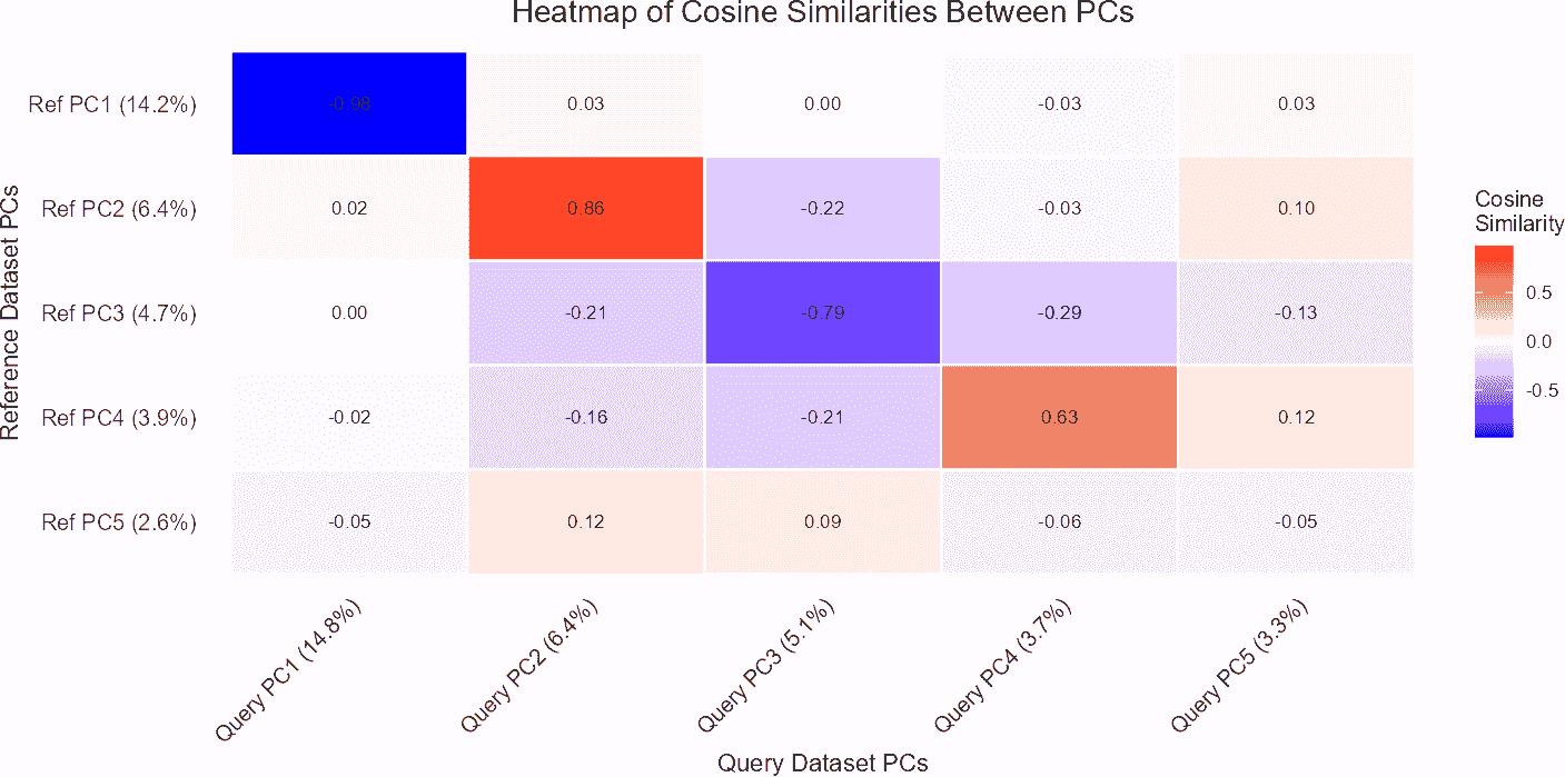
comparePCASubspace()
In single-cell RNA-seq analysis, it is essential to assess the
similarity between the subspaces spanned by the top principal components
(PCs) of query and reference datasets. This is particularly important
when comparing the structure and variation captured by each dataset. The
comparePCASubspace() function is designed to provide
insights into how well the subspaces align by computing the cosine
similarity between the loadings of the top variables for each PC. This
analysis helps in determining the degree of correspondence between the
datasets, which is critical for accurate cell type annotation and data
integration.
comparePCASubspace() performs the following
operations:
- Cosine Similarity Calculation: The function computes the cosine similarity between the loadings of the top variables for each PC in both the query and reference datasets. This similarity measures how closely the two datasets align in the space spanned by their principal components.
- Selection of Top Similarities: The function selects the top cosine similarity scores and stores the corresponding PC indices from both datasets. This step identifies the most aligned principal components between the two datasets.
- Variance Explained Calculation: It then calculates the average percentage of variance explained by the selected top PCs. This helps in understanding how much of the data’s variance is captured by these components.
- Weighted Cosine Similarity Score: Finally, the function computes a weighted cosine similarity score based on the top cosine similarities and the average percentage of variance explained. This score provides an overall measure of subspace alignment between the datasets.
# Compare PCA subspaces between query and reference data
subspace_comparison <- comparePCASubspace(
    query_data = query_data_cd4,
    reference_data = ref_data_cd4,
    query_cell_type_col = "expert_annotation",
    ref_cell_type_col = "expert_annotation",
    pc_subset = 1:5
)

# View weighted cosine similarity score
subspace_comparison$weighted_cosine_similarity
#> [1] 0.2620419

# Plot output for PCA subspace comparison (if a plot method is available)
plot(subspace_comparison)
In the results:
- Cosine Similarity: The values in principal_angles_cosines indicate the degree of alignment between the principal components of the query and reference datasets. Higher values suggest stronger alignment.
- Variance Explained: The average_variance_explained vector provides the average percentage of variance captured by the selected top PCs in both datasets. This helps assess the importance of these PCs in explaining data variation.
- Weighted Cosine Similarity: The weighted_cosine_similarity score combines the cosine similarity with variance explained to give a comprehensive measure of how well the subspaces align. A higher score indicates that the datasets are well-aligned in the PCA space.
By using comparePCASubspace(), you can quantify the
alignment of PCA subspaces between query and reference datasets, aiding
in the evaluation of dataset integration and the reliability of cell
type annotations.
plotPairwiseDistancesDensity()
Purpose
The plotPairwiseDistancesDensity() function is designed
to calculate and visualize the pairwise distances or correlations
between cell types in query and reference datasets. This function is
particularly useful in single-cell RNA sequencing (scRNA-seq) analysis,
where it is essential to evaluate the consistency and reliability of
cell type annotations by comparing their expression profiles.
Functionality
The function operates on SingleCellExperiment objects, which are commonly used to store single-cell data, including expression matrices and associated metadata. Users specify the cell types of interest in both the query and reference datasets, and the function computes either the distances or correlation coefficients between these cells.
When principal component analysis (PCA) is applied, the function projects the expression data into a lower-dimensional PCA space, which can be specified by the user. This allows for a more focused analysis of the major sources of variation in the data. Alternatively, if no dimensionality reduction is desired, the function can directly use the expression data for computation.
Depending on the user’s choice, the function can calculate pairwise Euclidean distances or correlation coefficients. The resulting values are used to compare the relationships between cells within the same dataset (either query or reference) and between cells across the two datasets.
Interpretation
The output of the function is a density plot generated by
ggplot2, which displays the distribution of pairwise
distances or correlations. The plot provides three key comparisons:
- Query vs. Query,
- Reference vs. Reference,
- Query vs. Reference.
By examining these density curves, users can assess the similarity of cells within each dataset and across datasets. For example, a higher density of lower distances in the “Query vs. Reference” comparison would suggest that the query and reference cells are similar in their expression profiles, indicating consistency in the annotation of the cell type across the datasets.
This visual approach offers an intuitive way to diagnose potential discrepancies in cell type annotations, identify outliers, or confirm the reliability of the cell type assignments.
# Example usage of the function
plotPairwiseDistancesDensity(query_data = query_data,
                             reference_data = reference_data,
                             query_cell_type_col = "expert_annotation",
                             ref_cell_type_col = "expert_annotation",
                             cell_type = "CD4",
                             pc_subset = 1:5,
                             distance_metric = "euclidean")
This example demonstrates how to compare CD4 cells between a query and reference dataset, with PCA applied to the first five principal components and pairwise Euclidean distances calculated. The output is a density plot that helps visualize the distribution of these distances, aiding in the interpretation of the similarity between the two datasets.
calculateWassersteinDistance()
the calculateWassersteinDistance() function uses the
concept of Wasserstein distances, a measure rooted in optimal transport
theory, to quantitatively compare these datasets. By projecting both
datasets into a common PCA space, the function enables a meaningful
comparison even when they originate from different experimental
conditions.
Before diving into a code example, it’s important to understand the output of this function. The result is a list containing three key components: the null distribution of Wasserstein distances computed from the reference dataset alone, the mean Wasserstein distance between the query and reference datasets, and a vector of the unique cell types present in the reference dataset. This comparison provides insights into how similar or different the query dataset is relative to the reference dataset.
What the function reveals is particularly valuable: if the mean Wasserstein distance between the query and reference is significantly different from the null distribution, it indicates a notable variation between the datasets, reflecting differences in cell-type compositions, technical artifacts, or biological questions of interest.
Code Example
# Generate the Wasserstein distance density plot
wasserstein_data <- calculateWassersteinDistance(
    query_data = query_data_cd4,
    reference_data = ref_data_cd4,
    query_cell_type_col = "expert_annotation",
    ref_cell_type_col = "expert_annotation",
    pc_subset = 1:10,
)
plot(wasserstein_data)
#> Picking joint bandwidth of 0.00906
The plotting function generates a density plot that provides a clear graphical representation of the Wasserstein distances. On the plot, you’ll see the distribution of Wasserstein distances calculated within the reference dataset, referred to as the null distribution.
Within this density plot, two significant vertical lines are overlayed: one representing the significance threshold and another indicating the mean Wasserstein distance between the reference and query datasets. The significance threshold is determined based on your specified alpha level, which is the probability threshold for considering differences between the datasets as statistically significant. This threshold line helps to establish a boundary; if the observed reference-query distance exceeds this threshold, it suggests that the differences between your query and reference datasets are unlikely to occur by random chance.
The line for the reference-query distance helps identify where this calculated distance lies in comparison to the null distribution. If this dashed line is noticeably separate from the bulk of the null distribution and beyond the significance threshold, it implies a significant deviation between the query dataset and the reference dataset. In practical terms, this could indicate distinct biological differences, batch effects, or other analytical artefacts that differentiate the datasets.
Statistical Measures to Assess Dataset Alignment
calculateCramerPValue()
The calculateCramerPValue function is designed to perform the Cramer test for comparing multivariate empirical cumulative distribution functions (ECDFs) between two samples in single-cell data. This test is particularly useful for assessing whether the distributions of principal components (PCs) differ significantly between the reference and query datasets for specific cell types.
To use this function, you first need to provide two key inputs:
reference_data and query_data, both of which
should be SingleCellExperiment
objects containing numeric expression matrices. If
query_data is not supplied, the function will only use the
reference_data. You should also specify the column names
for cell type annotations in both datasets via
ref_cell_type_col and query_cell_type_col. If
cell_types is not provided, the function will automatically
include all unique cell types found in the datasets. The
pc_subset parameter allows you to define which principal
components to include in the analysis, with the default being the first
five PCs.
The function performs the following steps: it first projects the data into PCA space, subsets the data according to the specified cell types and principal components, and then applies the Cramer test to compare the ECDFs between the reference and query datasets. The result is a named vector of p-values from the Cramer test for each cell type, which indicates whether there is a significant difference in the distributions of PCs between the two datasets.
Here’s an example of how to use the
calculateCramerPValue() function:
# Perform Cramer test for the specified cell types and principal components
cramer_test <- calculateCramerPValue(
    reference_data = reference_data,
    query_data = query_data,
    ref_cell_type_col = "expert_annotation",
    query_cell_type_col = "SingleR_annotation",
    cell_types = c("CD4", "CD8", "B_and_plasma", "Myeloid"),
    pc_subset = 1:5
)

# Display the Cramer test p-values
print(cramer_test)
#> B_and_plasma          CD4          CD8      Myeloid
#>   0.11788212   0.09090909   0.00000000   0.92007992
In this example, the function compares the distributions of the first five principal components between the reference and query datasets for cell types such as “CD4”, “CD8”, “B_and_plasma”, and “Myeloid”. The output is a vector of p-values indicating whether the differences in PC distributions are statistically significant.
calculateHotellingPValue()
The calculateHotellingPValue() function is designed to
compute Hotelling’s T-squared test statistic and corresponding p-values
for comparing multivariate means between reference and query datasets in
the context of single-cell RNA-seq data. This statistical test is
particularly useful for assessing whether the mean vectors of principal
components (PCs) differ significantly between the two datasets, which
can be indicative of differences in the cell type distributions.
To use this function, you need to provide two SingleCellExperiment
objects: query_data and reference_data, each
containing numeric expression matrices. You also need to specify the
column names for cell type annotations in both datasets with
query_cell_type_col and ref_cell_type_col. The
cell_types parameter allows you to choose which cell types
to include in the analysis, and if not specified, the function will
automatically include all cell types present in the datasets. The
pc_subset parameter determines which principal components
to consider, with the default being the first five PCs. Additionally,
n_permutation specifies the number of permutations for
calculating p-values, with a default of 500.
The function works by first projecting the data into PCA space and then performing Hotelling’s T-squared test for each specified cell type to compare the means between the reference and query datasets. It uses permutation testing to determine the p-values, indicating whether the observed differences in means are statistically significant. The result is a named numeric vector of p-values for each cell type.
Here is an example of how to use the
calculateHotellingPValue() function:
# Calculate Hotelling's T-squared test p-values
p_values <- calculateHotellingPValue(
    query_data = query_data,
    reference_data = reference_data,
    query_cell_type_col = "SingleR_annotation",
    ref_cell_type_col = "expert_annotation",
    pc_subset = 1:10
)

# Display the p-values rounded to five decimal places
print(round(p_values, 5))
#> B_and_plasma          CD4          CD8      Myeloid
#>        0.260        0.000        0.000        0.332
In this example, the function calculates p-values for Hotelling’s T-squared test, focusing on the first ten principal components to assess whether the multivariate means differ significantly between the reference and query datasets for each cell type. The p-values indicate the likelihood of observing the differences by chance and help identify significant disparities in cell type distributions.
calculateAveragePairwiseCorrelation()
The calculateAveragePairwiseCorrelation() function is
designed to compute the average pairwise correlations between specified
cell types in single-cell gene expression data. This function operates
on SingleCellExperiment
objects and is ideal for single-cell analysis workflows. It calculates
pairwise correlations between query and reference cells using a
specified correlation method, and then averages these correlations for
each cell type pair. This helps in assessing the similarity between
cells in the reference and query datasets and provides insights into the
reliability of cell type annotations.
To use the calculateAveragePairwiseCorrelation()
function, you need to supply it with two SingleCellExperiment
objects: one for the query cells and one for the reference cells. The
function also requires column names specifying cell type annotations in
both datasets, and optionally a vector of cell types to include in the
analysis. Additionally, you can specify a subset of principal components
to use, or use the raw data directly if pc_subset is set to
NULL. The correlation method can be either “spearman” or
“pearson”.
Here’s an example of how to use this function:
# Compute pairwise correlations between specified cell types
cor_matrix_avg <- calculateAveragePairwiseCorrelation(
  query_data = query_data,
  reference_data = reference_data,
  query_cell_type_col = "SingleR_annotation",
  ref_cell_type_col = "expert_annotation",
  cell_types = c("CD4", "CD8", "B_and_plasma"),
  pc_subset = 1:5,
  correlation_method = "spearman"
)

# Visualize the average pairwise correlation matrix
plot(cor_matrix_avg)
In this example, calculateAveragePairwiseCorrelation()
computes the average pairwise correlations for the cell types “CD4”,
“CD8”, and “B_and_plasma”. This function is particularly useful for
understanding the relationships between different cell types in your
single-cell datasets and evaluating how well cell types in the query
data correspond to those in the reference data.
regressPC()
The regressPC() function performs linear regression of a
covariate of interest onto one or more principal components using data
from a SingleCellExperiment
object. This method helps quantify the variance explained by a
covariate, which can be useful in applications such as quantifying batch
effects, assessing clustering homogeneity, and evaluating alignment
between query and reference datasets in cell type annotation
settings.
The function supports multiple regression scenarios depending on the data provided:
-
Query only: Regresses principal components against
cell types (
PC ~ cell_type) -
Query + Reference: Uses an interaction model to
assess annotation quality (
PC ~ cell_type * dataset)
When reference data is provided, the function projects query data onto the reference PCA space and performs unified interaction modeling to identify cell types with annotation inconsistencies between datasets.
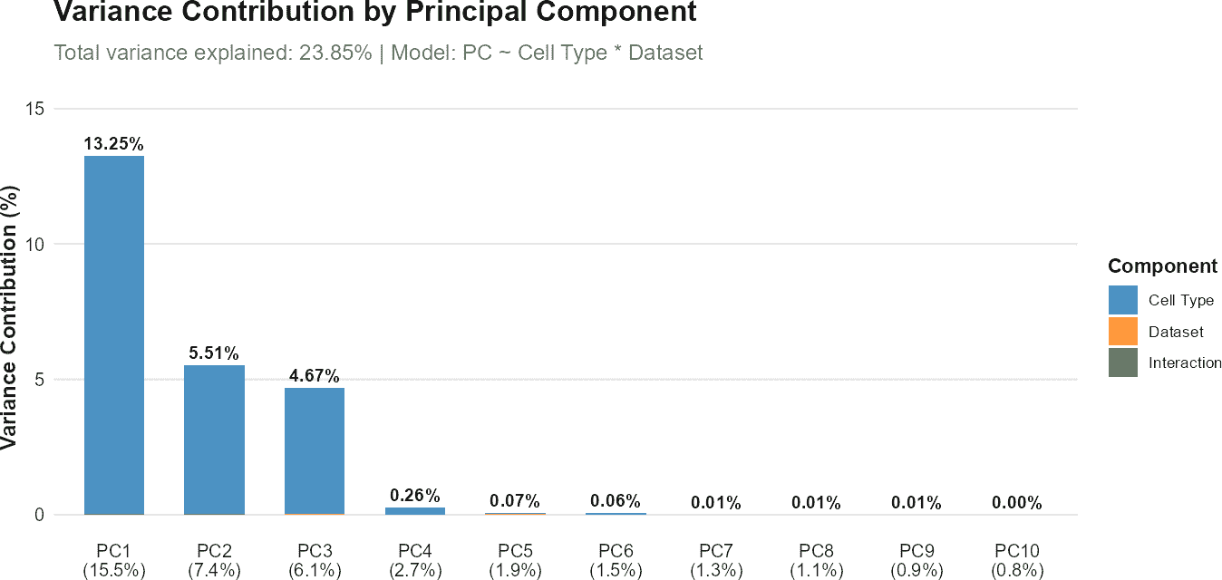
The function calculates the R-squared value from the linear regression for each principal component. For query-only analyses, variance contributions are computed as the product of the variance explained by each principal component and its corresponding R-squared value. The total variance explained by the covariate is obtained by summing these contributions across all principal components.
Here is how you can use the regressPC() function:
# Query-only analysis: How well do cell types separate in PCA space?
regress_res_query <- regressPC(
    query_data = query_data,
    query_cell_type_col = "expert_annotation",
    cell_types = c("CD4", "CD8", "B_and_plasma", "Myeloid"),
    pc_subset = 1:10
)

# Visualize results
plot(regress_res_query, plot_type = "r_squared")
plot(regress_res_query, plot_type = "variance_contribution")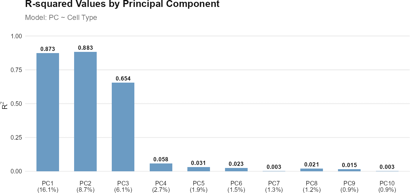

# Plot results showing p-values
plot(regress_res_query, plot_type = "coefficient_heatmap")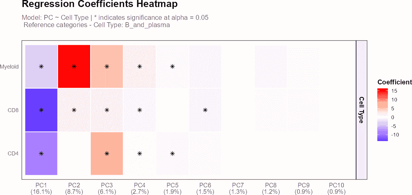
In this example, regressPC() is used to perform
regression analysis on principal components 1 to 10 from the query
dataset. The results are then visualized using plots showing the
R-squared values and cell type coefficients, with PC labels displaying
the percentage of variance explained by each component.
If you also have a reference dataset and want to assess annotation quality by comparing it with the query dataset, you can include it in the analysis:
# Perform regression analysis using both reference and query data
regress_res <- regressPC(
    query_data = query_data,
    reference_data = reference_data,
    query_cell_type_col = "SingleR_annotation",
    ref_cell_type_col = "expert_annotation",
    cell_types = c("CD4", "CD8", "B_and_plasma", "Myeloid"),
    pc_subset = 1:10
)

# Visualize results
plot(regress_res, plot_type = "r_squared")
plot(regress_res, plot_type = "variance_contribution")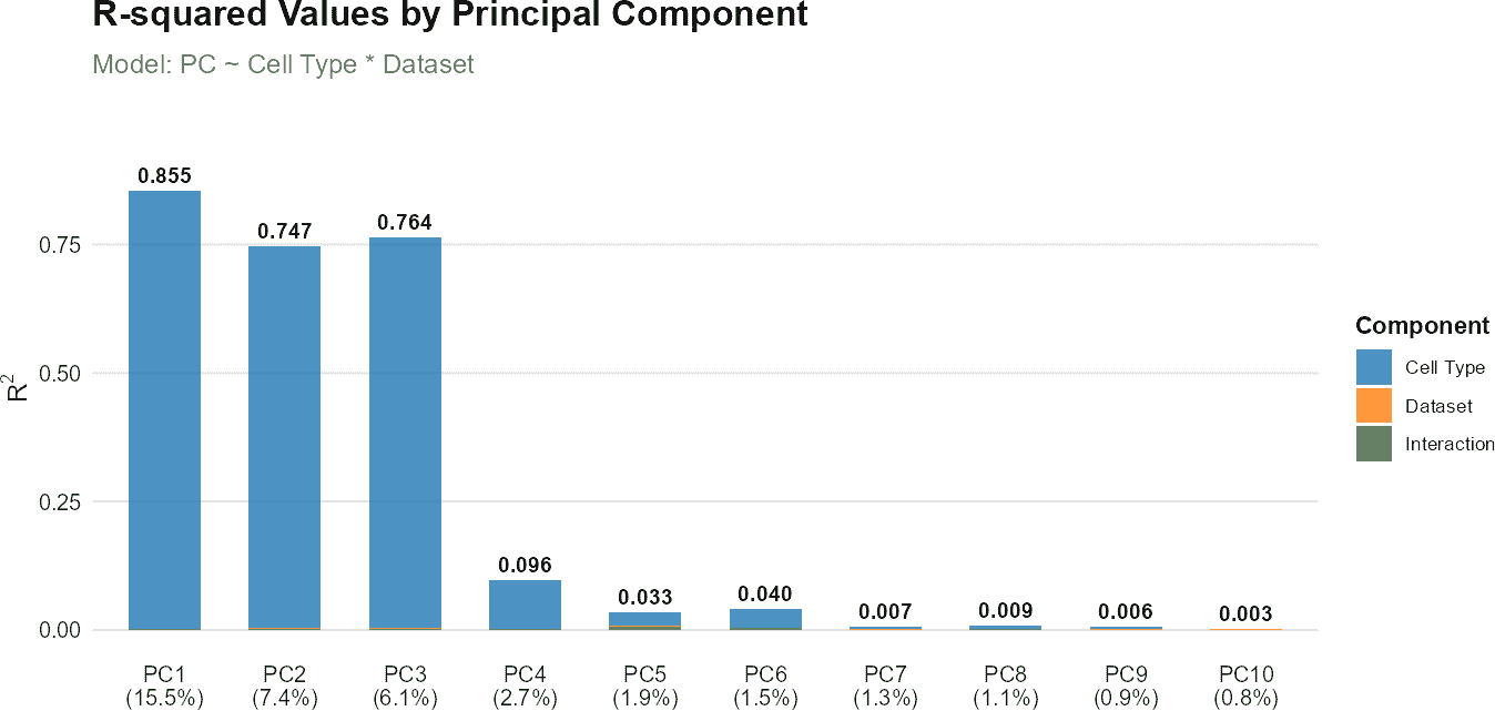
# Plot results showing p-values
plot(regress_res, plot_type = "coefficient_heatmap")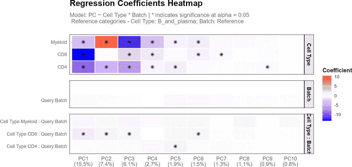
The regressPC() function also supports batch effect
analysis when sample or batch information is available. This capability
is particularly useful for assessing whether cell type annotations are
consistent across different batches or samples, and for identifying
batch-specific annotation problems.
When batch information is provided via the
query_batch_col parameter, the function performs different
regression analyses depending on the data configuration:
Query-only with Batch Information
For query data with multiple batches, the function fits an interaction model:
PC ~ cell_type × batch
This model captures: - Main effects of cell types:
How each cell type contributes to PC variation overall - Main
effects of batches: How each batch contributes to PC variation
overall
- Interaction effects: How cell type effects vary
across different batches
Large interaction effects indicate that certain cell types behave differently across batches, which could suggest batch-specific technical artifacts or genuine biological differences between samples.
Query + Reference with Batch Information
When both reference and query data are provided along with batch information, the analysis becomes more sophisticated. The function creates a unified batch labeling system where: - Reference data is labeled as “Reference” - Query batches are labeled as “Query_BatchName” (e.g., “Query_Sample1”, “Query_Sample2”)
The regression model then becomes:
PC ~ cell_type × batch
where the batch variable now includes both the reference and all query batches. This allows assessment of: - How consistently each cell type is annotated between reference and query datasets - Whether annotation quality varies across different query batches - Which specific query batches show the most deviation from reference annotations
Diagnostic Value
The interaction effects in batch analysis are particularly diagnostic: - Small interactions: Consistent cell type annotations across batches - Large interactions for specific cell types: Potential annotation problems in particular batches - Large interactions for specific batches: Systematic annotation issues in those batches
This analysis framework enables identification of batch-specific annotation problems and helps determine whether observed differences between datasets are due to technical batch effects or genuine biological variation.
Marker Gene Alignment
calculateHVGOverlap()
The calculateHVGOverlap() function computes the overlap
coefficient between two sets of highly variable genes (HVGs) from a
reference dataset and a query dataset. The overlap coefficient is a
measure of similarity between the two sets, reflecting how much the HVGs
in one dataset overlap with those in the other.
How the Function Operates
The function begins by ensuring that the input vectors
reference_genes and query_genes are character
vectors and that neither of them is empty. Once these checks are
complete, the function identifies the common genes between the two sets
using the intersect function, which finds the intersection of the two
gene sets.
Next, the function calculates the size of this intersection, representing the number of genes common to both sets. The overlap coefficient is then computed by dividing the size of the intersection by the size of the smaller set of genes. This ensures that the coefficient is a value between 0 and 1, where 0 indicates no overlap and 1 indicates complete overlap.
Finally, the function rounds the overlap coefficient to two decimal places before returning it as the output.
Interpretation
The overlap coefficient quantifies the extent to which the HVGs in the reference dataset align with those in the query dataset. A higher coefficient indicates a stronger similarity between the two datasets in terms of their HVGs, which can suggest that the datasets are more comparable or that they capture similar biological variability. Conversely, a lower coefficient indicates less overlap, suggesting that the datasets may be capturing different biological signals or that they are less comparable.
Code Example
# Load library to get top HVGs
library(scran)

# Select the top 500 highly variable genes from both datasets
ref_var_genes <- getTopHVGs(reference_data, n = 500)
#> Warning in getTopHVGs(reference_data, n = 500): 'getTopHVGs' is deprecated.
#> Use 'scrapper::chooseHighlyVariableGenes' instead.
#> See help("Deprecated")
#> Warning in fitTrendVar(fm, fv, ...): 'fitTrendVar' is deprecated.
#> Use 'scrapper::fitVarianceTrend' instead.
#> See help("Deprecated")
#> Warning in combineBlocks(collected, method = method, equiweight = equiweight, : 'combineBlocks' is deprecated.
#> See help("Deprecated")
query_var_genes <- getTopHVGs(query_data, n = 500)
#> Warning in getTopHVGs(query_data, n = 500): 'getTopHVGs' is deprecated.
#> Use 'scrapper::chooseHighlyVariableGenes' instead.
#> See help("Deprecated")
#> Warning in fitTrendVar(fm, fv, ...): 'fitTrendVar' is deprecated.
#> Use 'scrapper::fitVarianceTrend' instead.
#> See help("Deprecated")
#> Warning in combineBlocks(collected, method = method, equiweight = equiweight, : 'combineBlocks' is deprecated.
#> See help("Deprecated")

# Calculate the overlap coefficient between the reference and query HVGs
overlap_coefficient <- calculateHVGOverlap(reference_genes = ref_var_genes,
                                           query_genes = query_var_genes)

# Display the overlap coefficient
overlap_coefficient
#> [1] 0.93
calculateVarImpOverlap()
Overview
The calculateVarImpOverlap() function helps you identify
and compare the most important genes for distinguishing cell types in
both a reference dataset and a query dataset. It does this using the
Random Forest algorithm, which calculates how important each gene is in
differentiating between cell types.
Usage
To use the function, you need to provide a reference dataset containing expression data and cell type annotations. Optionally, you can also provide a query dataset if you want to compare gene importance across both datasets. The function allows you to specify which cell types to analyze and how many trees to use in the Random Forest model. Additionally, you can decide how many top genes you want to compare between the datasets.
Code Example
Let’s say you have a reference dataset (reference_data)
and a query dataset (query_data). Both datasets contain
expression data and cell type annotations, stored in columns named
“expert_annotation” and SingleR_annotation, respectively.
You want to calculate the importance of genes using 500 trees and
compare the top 50 genes between the datasets.
Here’s how you would use the function:
# RF function to compare which genes are best at differentiating cell types
rf_output <- calculateVarImpOverlap(reference_data = reference_data,
                                    query_data = query_data,
                                    query_cell_type_col = "expert_annotation",
                                    ref_cell_type_col = "expert_annotation",
                                    n_tree = 500,
                                    n_top = 50)

# Comparison table
rf_output$var_imp_comparison
#>              CD4-CD8     CD4-B_and_plasma          CD4-Myeloid
#>                 0.86                 0.82                 0.84
#>     CD8-B_and_plasma          CD8-Myeloid B_and_plasma-Myeloid
#>                 0.84                 0.84                 0.82
Interpretation:
After running the function, you’ll receive the importance scores of genes for each pair of cell types in your reference dataset. If you provided a query dataset, you’ll also get the importance scores for those cell types. The function will tell you how much the top genes in the reference and query datasets overlap, which helps you understand if the same genes are important for distinguishing cell types across different datasets.
For example, if there’s a high overlap, it suggests that similar genes are crucial in both datasets for differentiating the cell types, which could be important for validating your findings or identifying robust markers.
R Session Info
R version 4.6.1 (2026-06-24)
Platform: x86_64-pc-linux-gnu
Running under: Ubuntu 24.04.4 LTS

Matrix products: default
BLAS:   /usr/lib/x86_64-linux-gnu/openblas-pthread/libblas.so.3
LAPACK: /usr/lib/x86_64-linux-gnu/openblas-pthread/libopenblasp-r0.3.26.so;  LAPACK version 3.12.0

locale:
 [1] LC_CTYPE=C.UTF-8       LC_NUMERIC=C           LC_TIME=C.UTF-8
 [4] LC_COLLATE=C.UTF-8     LC_MONETARY=C.UTF-8    LC_MESSAGES=C.UTF-8
 [7] LC_PAPER=C.UTF-8       LC_NAME=C              LC_ADDRESS=C
[10] LC_TELEPHONE=C         LC_MEASUREMENT=C.UTF-8 LC_IDENTIFICATION=C

time zone: UTC
tzcode source: system (glibc)

attached base packages:
[1] stats4    stats     graphics  grDevices utils     datasets  methods
[8] base

other attached packages:
 [1] scater_1.40.2               ggplot2_4.0.3
 [3] scran_1.40.0                scuttle_1.22.0
 [5] SingleCellExperiment_1.34.0 SummarizedExperiment_1.42.0
 [7] Biobase_2.72.0              GenomicRanges_1.64.0
 [9] Seqinfo_1.2.0               IRanges_2.46.0
[11] S4Vectors_0.50.1            BiocGenerics_0.58.1
[13] generics_0.1.4              MatrixGenerics_1.24.0
[15] matrixStats_1.5.0           scDiagnostics_1.7.2
[17] BiocStyle_2.40.0

loaded via a namespace (and not attached):
 [1] tidyselect_1.2.1    viridisLite_0.4.3   vipor_0.4.7
 [4] dplyr_1.2.1         farver_2.1.2        viridis_0.6.5
 [7] S7_0.2.2            fastmap_1.2.0       bluster_1.22.0
[10] transport_0.15-4    digest_0.6.39       rsvd_1.0.5
[13] lifecycle_1.0.5     cluster_2.1.8.2     statmod_1.5.2
[16] magrittr_2.0.5      compiler_4.6.1      rlang_1.3.0
[19] sass_0.4.10         tools_4.6.1         igraph_2.3.3
[22] yaml_2.3.12         data.table_1.18.4   knitr_1.51
[25] labeling_0.4.3      S4Arrays_1.12.0     dqrng_0.4.1
[28] htmlwidgets_1.6.4   DelayedArray_0.38.2 RColorBrewer_1.1-3
[31] abind_1.4-8         BiocParallel_1.46.0 withr_3.0.3
[34] desc_1.4.3          grid_4.6.1          cramer_0.9-4
[37] beachmat_2.28.0     edgeR_4.10.1        scales_1.4.0
[40] ggridges_0.5.7      cli_3.6.6           rmarkdown_2.31
[43] ragg_1.5.2          otel_0.2.0          metapod_1.20.0
[46] ggbeeswarm_0.7.3    cachem_1.1.0        stringr_1.6.0
[49] parallel_4.6.1      BiocManager_1.30.27 XVector_0.52.0
[52] vctrs_0.7.3         boot_1.3-32         Matrix_1.7-5
[55] jsonlite_2.0.0      bookdown_0.47       BiocSingular_1.28.0
[58] BiocNeighbors_2.6.0 ggrepel_0.9.8       beeswarm_0.4.0
[61] irlba_2.3.7         systemfonts_1.3.2   locfit_1.5-9.12
[64] limma_3.68.4        jquerylib_0.1.4     glue_1.8.1
[67] pkgdown_2.2.0       codetools_0.2-20    stringi_1.8.7
[70] gtable_0.3.6        ScaledMatrix_1.20.0 tibble_3.3.1
[73] pillar_1.11.1       htmltools_0.5.9     R6_2.6.1
[76] textshaping_1.0.5   evaluate_1.0.5      lattice_0.22-9
[79] bslib_0.11.0        Rcpp_1.1.2          gridExtra_2.3.1
[82] SparseArray_1.12.2  ranger_0.18.0       xfun_0.59
[85] fs_2.1.0            pkgconfig_2.0.3