Detection and Analysis of Annotation Anomalies

Anthony Christidis

Core for Computational Biomedicine, Harvard Medical School

Andrew Ghazi

Core for Computational Biomedicine, Harvard Medical School

Smriti Chawla

Core for Computational Biomedicine, Harvard Medical School

Nitesh Turaga

Core for Computational Biomedicine, Harvard Medical School

Ludwig Geistlinger

Core for Computational Biomedicine, Harvard Medical School

Robert Gentleman

Core for Computational Biomedicine, Harvard Medical School
Source: vignettes/AnnotationAnomalies.Rmd

AnnotationAnomalies.Rmd

Introduction

The scDiagnostics package provides powerful tools for anomaly detection in single-cell data, enabling researchers to identify and analyze outliers in complex datasets. Central to this process is the detectAnomaly() function, which integrates dimensionality reduction through Principal Component Analysis (PCA) with the robust capabilities of the isolation forest algorithm.

In single-cell analysis, detecting anomalies is crucial for identifying potential data issues, such as mislabeled cells, technical artifacts, or biologically distinct subpopulations. The detectAnomaly() function offers a versatile approach to anomaly detection by allowing users to project data onto a PCA space and apply isolation forests to uncover outliers. Whether working solely with a reference dataset or comparing a query dataset against a well-characterized reference, this function provides detailed insights into potential anomalies.

This vignette illustrates how to effectively use the detectAnomaly() function in various scenarios. We explore both cell-type-specific and global anomaly detection, demonstrate the utility of integrating query data with reference data, and offer guidance on interpreting the results. Additionally, we show how to extend this analysis by combining anomaly detection with PCA loadings using the calculateCellSimilarityPCA() function, providing a comprehensive toolkit for investigating the structure and quality of single-cell data.

This vignette also demonstrates the use of two functions, calculateCellDistances() and calculateCellDistancesSimilarity(), to analyze the distances between cells in query and reference datasets and to measure the similarity of density distributions. These functions are useful for investigating how cells in different datasets relate to each other, particularly in the context of identifying anomalies and understanding distribution overlaps.

Preliminaries

In the context of the scDiagnostics package, the following datasets illustrate the application of these tools:

reference_data: A curated and processed dataset containing expert-assigned cell type annotations. This dataset serves as a reference for comparison and can be used alone to detect anomalies within the reference annotations.
query_data: A dataset that also includes expert-assigned cell type annotations, but additionally features annotations generated by the SingleR package. This allows for the comparison of expert annotations with those produced by an automated method to detect inconsistencies or anomalies.

# Load library
library(scDiagnostics)

# Load datasets
data("reference_data")
data("query_data")

# Set seed for reproducibility
set.seed(0)

By using these datasets, you can leverage the package’s tools to compare annotations between reference_data and query_data, or analyze reference_data alone to identify potential issues. The package’s flexibility supports various analysis scenarios, whether you need to assess overall annotation quality or focus on specific cell types.

Through these capabilities, scDiagnostics empowers you to perform thorough and nuanced assessments of cell type annotations, enhancing the accuracy and reliability of your analyses.

The `detectAnomaly()` Function

Function Overview

Description

The detectAnomaly() function integrates dimensionality reduction via PCA with the isolation forest algorithm to detect anomalies in single-cell data. By projecting both reference and query datasets (if available) onto the PCA space of the reference data, the function trains an isolation forest model on reference data in PCA space to pinpoint anomalies in the reference or query data. This approach is highly versatile:

Reference Only: Compute anomaly scores solely for the reference dataset to identify potential issues within the reference itself.
Reference and Query: Compare the query dataset against the reference to find anomalies in the query data that may not align with the established reference.
Global and Specific Analysis: Assess anomalies at a global level or focus on specific cell types to gain targeted insights into your data. The function also provides detailed visualizations and statistical outputs to help you interpret the anomalies detected.

Parameters

The function takes a SingleCellExperiment object as reference_data and trains an isolation forest model on the reference PCA-projected data, with an optional query_data for projecting onto this PCA space for anomaly detection. You can specify cell type annotations through ref_cell_type_col and query_cell_type_col, and limit the analysis to certain cell types using the cell_types parameter. The function allows you to select specific principal components to use to train the isolation forest via pc_subset, adjust the number of trees with n_tree, and set an anomaly_threshold for classifying anomalies.

Return Value

The function returns several outputs: anomaly_scores indicating the likelihood of each cell being an anomaly, a logical vector (anomaly) identifying these anomalies, PCA projections for the reference data (reference_mat_subset) and optionally for the query data (query_mat_subset), and the proportion of variance explained by the selected principal components (var_explained).

`detectAnomaly()` Examples

Anomaly Detection with Reference and Query Data

This section demonstrates how to use the detectAnomaly() function when both reference and query datasets are provided. It includes examples of analyzing anomalies for specific cell types and globally across all data.

Example 1: Cell-Type Specific Anomaly Detection

In this example, we analyze anomalies specifically for the “CD4” cell type. The anomaly scores are trained on the PCA projections of the “CD4” cells from the reference dataset. If query data is provided, anomaly scores for the query data are predicted based on the PCA projections of the query data onto the reference PCA space for the “CD4” cell type.

# Perform anomaly detection
anomaly_output <- detectAnomaly(reference_data = reference_data, 
                                query_data = query_data, 
                                ref_cell_type_col = "expert_annotation", 
                                query_cell_type_col = "SingleR_annotation",
                                pc_subset = 1:5,
                                n_tree = 500,
                                anomaly_treshold = 0.6)

# Plot the output for the "CD4" cell type
plot(anomaly_output, 
     cell_type = "CD4", 
     pc_subset = 1:5, 
     data_type = "query")

Example 2: Global Anomaly Detection

Here, we perform global anomaly detection by setting cell_type = NULL. In this case, the isolation forest is trained on PCA projections of all cells in the reference data combined. The global anomaly scores are then computed for both reference and query datasets.

# Perform anomaly detection
anomaly_output <- detectAnomaly(reference_data = reference_data, 
                                query_data = query_data, 
                                ref_cell_type_col = "expert_annotation", 
                                query_cell_type_col = "SingleR_annotation",
                                pc_subset = 1:5,
                                n_tree = 500,
                                anomaly_treshold = 0.6)

# Plot the global anomaly scores
plot(anomaly_output, 
     cell_type = NULL,  # Plot all cell types
     pc_subset = 1:5, 
     data_type = "query")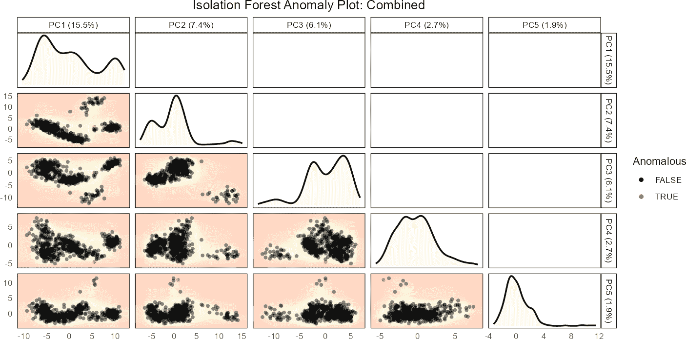

Setting cell_type = NULL means that the anomaly detection is done globally. The isolation forest is trained on PCA projections of all cells from the reference dataset. Anomaly scores are then predicted for the query data based on these global PCA projections. The plot provides a comprehensive view of anomalies across all cell types in the query dataset.

Anomaly Detection on Reference Data

Note that if you do not provide a query dataset to the detectAnomaly() function, the function will only return the anomaly output data on the reference data.

Integrating Anomaly Detection with Cell Similarity Analysis Using PCA Loadings

The detectAnomaly() function identifies anomalous cells in a dataset by detecting outliers based on PCA results. Once anomalies are detected, calculateCellSimilarityPCA() evaluates how these outliers influence principal component directions. This analysis helps determine if anomalous cells significantly impact later PCs, which capture finer variations in the data. By combining these functions, you can both pinpoint anomalies and understand their effect on PCA directions, providing deeper insights into the data structure.

# Detect anomalies and select top anomalies for further analysis
anomaly_output <- detectAnomaly(reference_data = reference_data, 
                                query_data = query_data,
                                ref_cell_type_col = "expert_annotation", 
                                query_cell_type_col = "SingleR_annotation",
                                pc_subset = 1:10,
                                n_tree = 500,
                                anomaly_treshold = 0.5)

# Select the top 6 anomalies based on the anomaly scores
top6_anomalies <- names(sort(anomaly_output$Combined$reference_anomaly_scores, 
                             decreasing = TRUE)[1:6])

# Calculate cosine similarity between the top anomalies and top 25 PCs
cosine_similarities <- calculateCellSimilarityPCA(reference_data, 
                                                  cell_names = top6_anomalies, 
                                                  pc_subset = 1:25, 
                                                  n_top_vars = 50)

# Plot the cosine similarities across PCs
round(cosine_similarities[, paste0("PC", 15:25)], 2)
#>                    PC15  PC16  PC17  PC18  PC19  PC20  PC21  PC22  PC23  PC24
#> ACACCAATCTTAACCT-1 0.10 -0.05  0.24  0.01 -0.05 -0.08  0.16 -0.15  0.01 -0.08
#> GGCTGGTAGCCAACAG-1 0.06  0.13  0.33 -0.06 -0.13  0.03  0.07 -0.01  0.11 -0.04
#> TACACGAAGCGATAGC-1 0.07  0.02 -0.01  0.12  0.16  0.02 -0.08  0.14 -0.06  0.26
#> CATGGCGCATGCTGGC-1 0.13 -0.12  0.08  0.14 -0.24 -0.03 -0.01 -0.17 -0.17  0.05
#> GTACTTTTCCGTTGTC-1 0.16  0.01  0.24 -0.03 -0.02 -0.04 -0.11 -0.08 -0.15  0.16
#> ATTTCTGAGCGATATA-1 0.05  0.29  0.24  0.18 -0.20  0.05 -0.15  0.08  0.15 -0.11
#>                    PC25
#> ACACCAATCTTAACCT-1 0.01
#> GGCTGGTAGCCAACAG-1 0.26
#> TACACGAAGCGATAGC-1 0.36
#> CATGGCGCATGCTGGC-1 0.01
#> GTACTTTTCCGTTGTC-1 0.17
#> ATTTCTGAGCGATATA-1 0.06

Note that there is also a plot method for the object return for calculateCellSimilarityPCA(). See reference manual for details.

Analyzing Cell Distances

`calculateCellDistances()`

The calculateCellDistances() function calculates Euclidean distances between cells within the reference dataset and between query cells and reference cells. This helps in understanding how closely related cells are within and across datasets based on their principal component (PC) scores.

Function Usage

# Compute cell distances
distance_data <- calculateCellDistances(
    query_data = query_data,
    reference_data = reference_data,
    query_cell_type_col = "SingleR_annotation",
    ref_cell_type_col = "expert_annotation",
    pc_subset = 1:10
)

In the code above:

query_data and reference_data: These are SingleCellExperiment objects containing the respective datasets for analysis.
query_cell_type_col and ref_cell_type_col: These arguments specify the columns in the colData of each dataset that contain cell type annotations.
pc_subset: Specifies which principal components (1 to 10) are used to compute distances. PCA is applied for dimensionality reduction before calculating distances.

Output

The output distance_data is a list where each entry contains:

ref_distances: Pairwise distances within the reference dataset for each cell type.
query_to_ref_distances: Distances from each query cell to all reference cells for each cell type.

Example Workflow

In the example workflow, the first step involves plotting the distributions of cell distances for selected query cells against various reference cell populations. This involves visualizing both the distances between the query cells and the reference cells as well as the distances among the reference cells themselves. For each cell type, such as CD4 and CD8, these plots illustrate how the selected query cells compare in terms of their proximity to different reference populations.

# Identify top 6 anomalies for CD4 cells
cd4_anomalies <- detectAnomaly(
  reference_data = reference_data,
  query_data = query_data,
  query_cell_type_col = "SingleR_annotation",
  ref_cell_type_col = "expert_annotation",
  pc_subset = 1:10,
  n_tree = 500,
  anomaly_treshold = 0.5)

# Top 6 CD4 anomalies
cd4_top6_anomalies <- names(sort(cd4_anomalies$CD4$query_anomaly_scores, decreasing = TRUE)[1:6])

# Plot distances for CD4 and CD8 cells
plot(distance_data, ref_cell_type = "CD4", cell_names = cd4_top6_anomalies)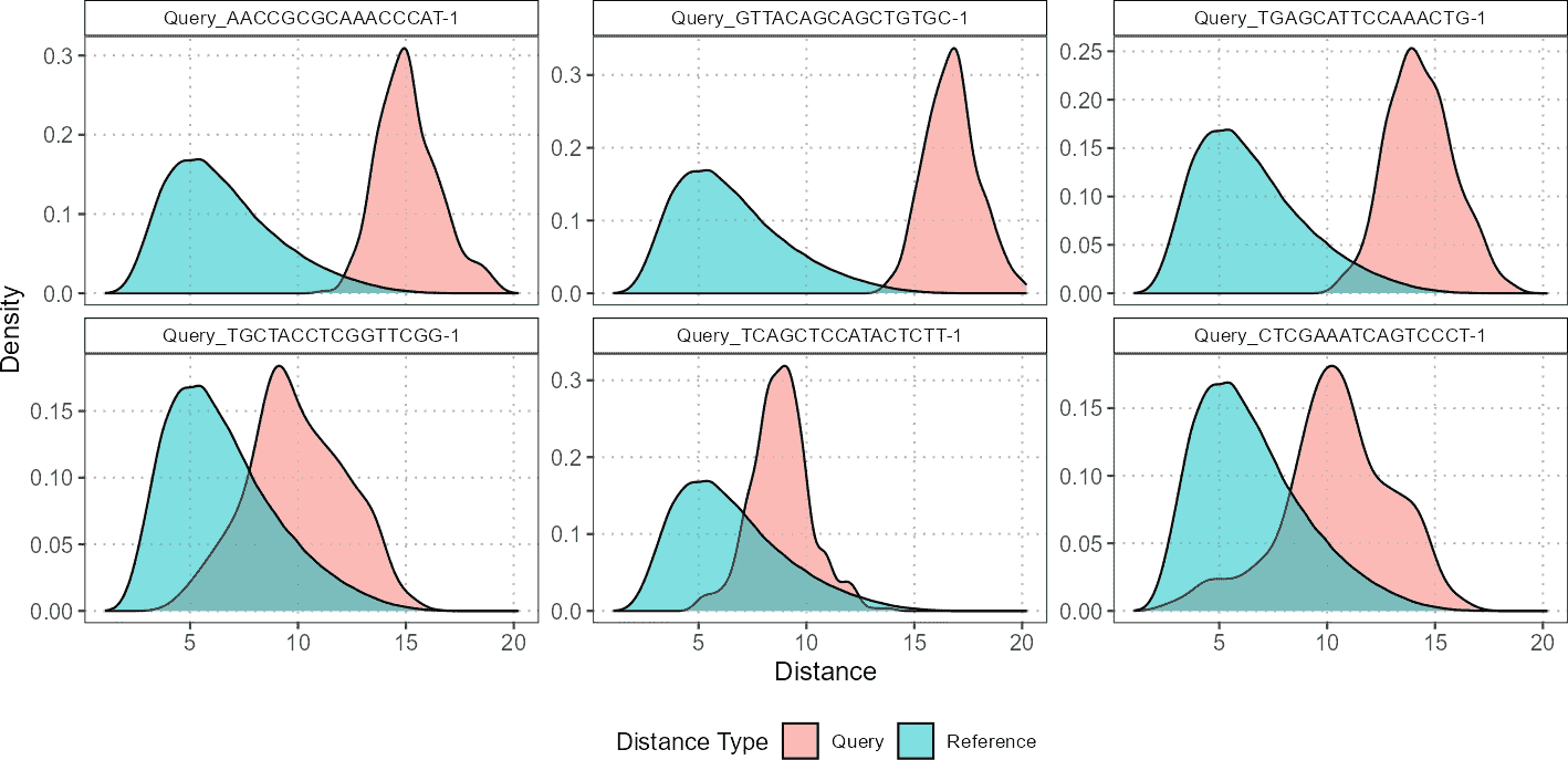

For CD4 cells, you might observe that the query cells are located much further away from the reference cells, indicating a significant divergence in their density distributions. This suggests that the CD4 query cells are less similar to the CD4 reference cells, showing greater variation or potential anomalies.

In contrast, for CD8 cells, the plots might reveal more overlap between the density distributions of query cells and reference cells. This overlap indicates that the CD8 query cells are more similar to the CD8 reference cells, suggesting better alignment or less divergence between their densities. Such insights are crucial for understanding how closely the query cells match with reference populations and can help in identifying cell types with notable differences or similarities.

# Plot distances for CD8 cells
plot(distance_data, ref_cell_type = "CD8", cell_names = cd4_top6_anomalies)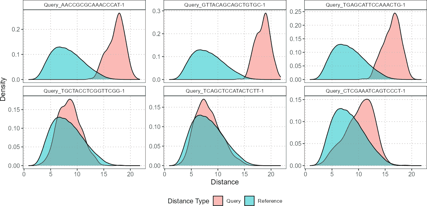

`calculateCellDistancesSimilarity()`

The calculateCellDistancesSimilarity() function measures how similar the density distributions of query cells are to those in the reference dataset. It computes Bhattacharyya coefficients and Hellinger distances, which quantify the overlap between the distributions.

The Bhattacharyya coefficient and Hellinger distance are two measures used to quantify the similarity between probability distributions. The Bhattacharyya coefficient ranges from 0 to 1, where a value closer to 1 indicates higher similarity between distributions, while a value closer to 0 suggests greater dissimilarity. The Hellinger distance, also ranging from 0 to 1, reflects the divergence between distributions, with lower values indicating greater similarity and higher values showing more distinct distributions. In the context of comparing query cells to reference cells, a high Bhattacharyya coefficient and a low Hellinger distance both suggest that the query cells have density profiles similar to those in the reference dataset, which can be desirable depending on the experimental objectives.

# Compute similarity measures for top 6 CD4 anomalies
overlap_measures <- calculateCellDistancesSimilarity(
  query_data = query_data,
  reference_data = reference_data,
  cell_names = cd4_top6_anomalies,
  query_cell_type_col = "SingleR_annotation",
  ref_cell_type_col = "expert_annotation",
  pc_subset = 1:10)
overlap_measures
#> $bhattacharyya_coef
#>                 Cell       CD4       CD8 B_and_plasma   Myeloid
#> 1 TTGGAACTCGCTTAGA-1 0.4664148 0.9678914    0.3587941 0.2574115
#> 2 GATCGCGTCCCATTAT-1 0.6695226 0.9709480    0.3327168 0.2051765
#> 3 AGCATACGTTGAGTTC-1 0.6526016 0.9609405    0.3085990 0.2102890
#> 4 TAAGCGTGTAATCGTC-1 0.6049953 0.9677820    0.3331004 0.1622547
#> 5 CCATGTCTCGTCTGCT-1 0.6158507 0.9812964    0.3421234 0.2000697
#> 6 TGCCCTAAGCGGCTTC-1 0.6184935 0.9558004    0.3118239 0.1380546
#> 
#> $hellinger_dist
#>                 Cell       CD4       CD8 B_and_plasma   Myeloid
#> 1 TTGGAACTCGCTTAGA-1 0.7304692 0.1791887    0.8007534 0.8617357
#> 2 GATCGCGTCCCATTAT-1 0.5748716 0.1704463    0.8168741 0.8915288
#> 3 AGCATACGTTGAGTTC-1 0.5894051 0.1976348    0.8315053 0.8886569
#> 4 TAAGCGTGTAATCGTC-1 0.6284940 0.1794938    0.8166392 0.9152843
#> 5 CCATGTCTCGTCTGCT-1 0.6197978 0.1367610    0.8110959 0.8943882
#> 6 TGCCCTAAGCGGCTTC-1 0.6176621 0.2102369    0.8295638 0.9284102

R Session Info

R version 4.4.1 (2024-06-14)
Platform: x86_64-pc-linux-gnu
Running under: Ubuntu 22.04.5 LTS

Matrix products: default
BLAS:   /usr/lib/x86_64-linux-gnu/openblas-pthread/libblas.so.3 
LAPACK: /usr/lib/x86_64-linux-gnu/openblas-pthread/libopenblasp-r0.3.20.so;  LAPACK version 3.10.0

locale:
 [1] LC_CTYPE=C.UTF-8       LC_NUMERIC=C           LC_TIME=C.UTF-8       
 [4] LC_COLLATE=C.UTF-8     LC_MONETARY=C.UTF-8    LC_MESSAGES=C.UTF-8   
 [7] LC_PAPER=C.UTF-8       LC_NAME=C              LC_ADDRESS=C          
[10] LC_TELEPHONE=C         LC_MEASUREMENT=C.UTF-8 LC_IDENTIFICATION=C   

time zone: UTC
tzcode source: system (glibc)

attached base packages:
[1] stats     graphics  grDevices utils     datasets  methods   base     

other attached packages:
[1] scDiagnostics_1.1.0 BiocStyle_2.32.1   

loaded via a namespace (and not attached):
 [1] SummarizedExperiment_1.34.0 gtable_0.3.6               
 [3] xfun_0.48                   bslib_0.8.0                
 [5] ggplot2_3.5.1               htmlwidgets_1.6.4          
 [7] Biobase_2.64.0              lattice_0.22-6             
 [9] generics_0.1.3              vctrs_0.6.5                
[11] tools_4.4.1                 parallel_4.4.1             
[13] stats4_4.4.1                tibble_3.2.1               
[15] fansi_1.0.6                 pkgconfig_2.0.3            
[17] Matrix_1.7-0                desc_1.4.3                 
[19] S4Vectors_0.42.1            ggridges_0.5.6             
[21] lifecycle_1.0.4             GenomeInfoDbData_1.2.12    
[23] farver_2.1.2                compiler_4.4.1             
[25] textshaping_0.4.0           munsell_0.5.1              
[27] GenomeInfoDb_1.40.1         htmltools_0.5.8.1          
[29] sass_0.4.9                  yaml_2.3.10                
[31] pkgdown_2.1.1               pillar_1.9.0               
[33] crayon_1.5.3                jquerylib_0.1.4            
[35] SingleCellExperiment_1.26.0 DelayedArray_0.30.1        
[37] cachem_1.1.0                abind_1.4-8                
[39] tidyselect_1.2.1            digest_0.6.37              
[41] dplyr_1.1.4                 bookdown_0.41              
[43] labeling_0.4.3              fastmap_1.2.0              
[45] grid_4.4.1                  colorspace_2.1-1           
[47] cli_3.6.3                   SparseArray_1.4.8          
[49] magrittr_2.0.3              S4Arrays_1.4.1             
[51] utf8_1.2.4                  withr_3.0.2                
[53] UCSC.utils_1.0.0            scales_1.3.0               
[55] rmarkdown_2.28              XVector_0.44.0             
[57] httr_1.4.7                  matrixStats_1.4.1          
[59] ragg_1.3.3                  isotree_0.6.1-1            
[61] evaluate_1.0.1              knitr_1.48                 
[63] GenomicRanges_1.56.2        IRanges_2.38.1             
[65] rlang_1.1.4                 Rcpp_1.0.13                
[67] glue_1.8.0                  BiocManager_1.30.25        
[69] BiocGenerics_0.50.0         jsonlite_1.8.9             
[71] R6_2.5.1                    MatrixGenerics_1.16.0      
[73] systemfonts_1.1.0           fs_1.6.4                   
[75] zlibbioc_1.50.0

Detection and Analysis of Annotation Anomalies

Anthony Christidis

Andrew Ghazi

Smriti Chawla

Nitesh Turaga

Ludwig Geistlinger

Robert Gentleman

Introduction

Preliminaries

The detectAnomaly() Function

Function Overview

Description

Parameters

Return Value

detectAnomaly() Examples

Anomaly Detection with Reference and Query Data

Example 1: Cell-Type Specific Anomaly Detection

Example 2: Global Anomaly Detection

Anomaly Detection on Reference Data

Integrating Anomaly Detection with Cell Similarity Analysis Using PCA Loadings

Analyzing Cell Distances

calculateCellDistances()

Function Usage

Output

Example Workflow

calculateCellDistancesSimilarity()

R Session Info

The `detectAnomaly()` Function

`detectAnomaly()` Examples

`calculateCellDistances()`

`calculateCellDistancesSimilarity()`