Project Query Data onto a Unified Discriminant Space of Reference Data

This function projects query single-cell RNA-seq data onto a unified discriminant space defined by reference data. The reference data is used to identify important variables across all cell types and compute discriminant vectors, which are then used to project both reference and query data. Similarity between the query and reference projections can be assessed using cosine similarity and Mahalanobis distance.

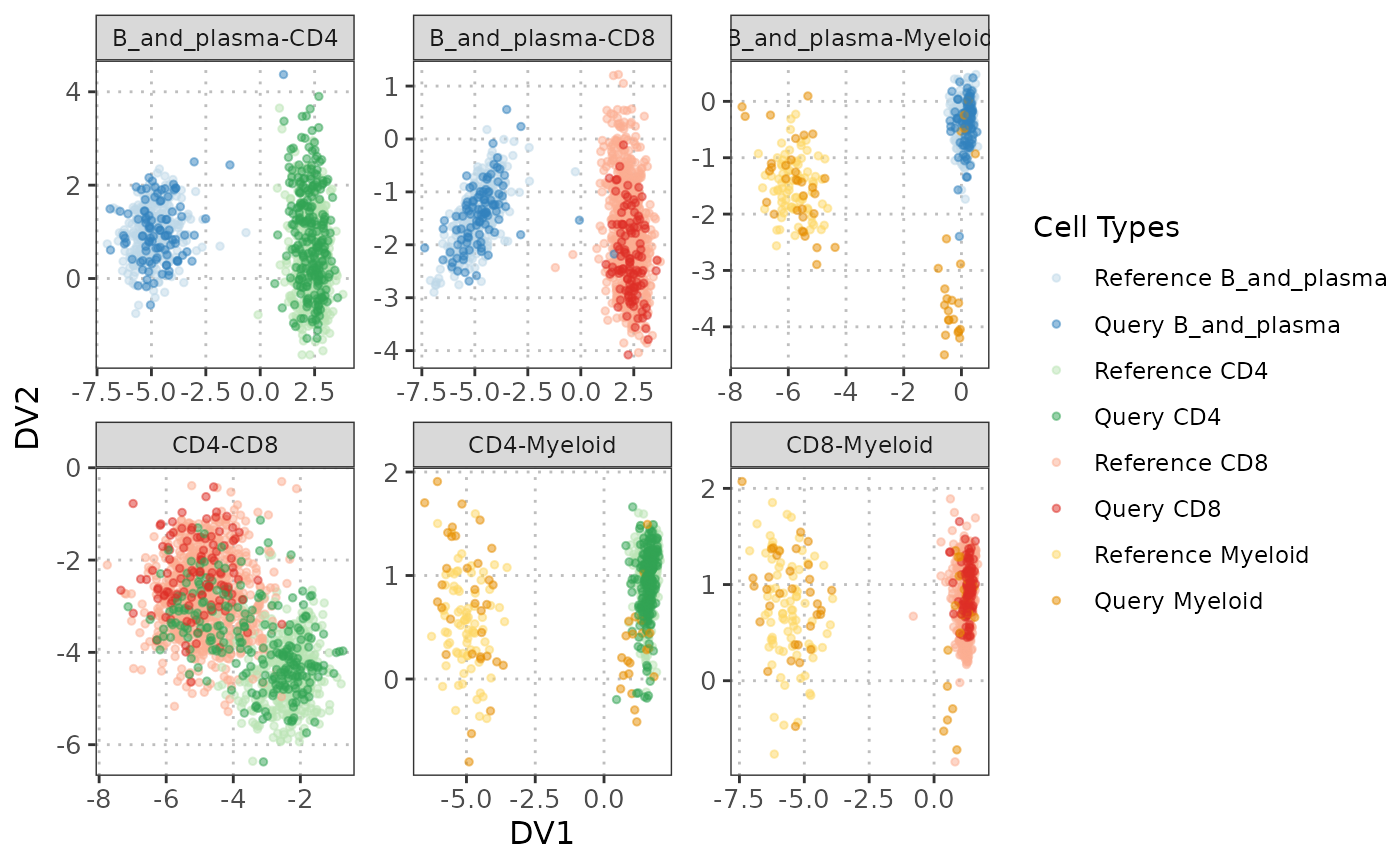
The S3 plot method visualizes the projected reference and query data on the unified discriminant space.

calculateDiscriminantSpace(
  reference_data,
  query_data = NULL,
  ref_cell_type_col,
  query_cell_type_col = NULL,
  cell_types = NULL,
  n_tree = 500,
  n_top = 20,
  eigen_threshold = 0.1,
  calculate_metrics = FALSE,
  alpha = 0.01,
  assay_name = "logcounts"
)

# S3 method for class 'calculateDiscriminantSpaceObject'
plot(
  x,
  cell_types = NULL,
  dv_subset = NULL,
  lower_facet = c("scatter", "contour", "ellipse", "blank"),
  diagonal_facet = c("ridge", "density", "boxplot", "blank"),
  upper_facet = c("blank", "scatter", "contour", "ellipse"),
  ...
)

Arguments

reference_data: A SingleCellExperiment object containing numeric expression matrix for the reference cells.
query_data: A SingleCellExperiment object containing numeric expression matrix for the query cells. If NULL, only the projected reference data is returned. Default is NULL.
ref_cell_type_col: The column name in reference_data indicating cell type labels.
query_cell_type_col: The column name in query_data indicating cell type labels.
cell_types: A character vector specifying the cell types to plot. If NULL (default), all cell types will be plotted.
n_tree: An integer specifying the number of trees for the random forest used in variable importance calculation.
n_top: An integer specifying the number of top variables to select based on importance scores from each pairwise comparison.
eigen_threshold: A numeric value specifying the threshold for retaining eigenvalues in discriminant analysis.
calculate_metrics: Parameter to determine if cosine similarity and Mahalanobis distance metrics should be computed. Default is FALSE.
alpha: A numeric value specifying the significance level for Mahalanobis distance cutoff.
assay_name: Name of the assay on which to perform computations. Default is "logcounts".
x: An object of class calculateDiscriminantSpaceObject containing the projected data on the discriminant space.
dv_subset: A numeric vector specifying which discriminant vectors to include in the plot. Default is the number of cell types minus 1.
lower_facet: Type of plot to use for the lower panels. Either "scatter" (default), "contour", "ellipse", or "blank".
diagonal_facet: Type of plot to use for the diagonal panels. Either "ridge" (default), "density", "boxplot" or "blank".
upper_facet: Type of plot to use for the upper panels. Either "blank" (default), "scatter", "contour", or "ellipse".
...: Additional arguments to be passed to the plotting functions.

Value

A list with the following components:

discriminant_eigenvalues: Eigenvalues from the discriminant analysis.
discriminant_eigenvectors: Eigenvectors from the discriminant analysis.
ref_proj: Reference data projected onto the discriminant space.
query_proj: Query data projected onto the discriminant space (if query_data is provided).
query_mahalanobis_dist: Mahalanobis distances of query projections (if calculate_metrics is TRUE).
mahalanobis_crit: Cutoff value for Mahalanobis distance significance (if calculate_metrics is TRUE).
query_cosine_similarity: Cosine similarity scores of query projections (if calculate_metrics is TRUE).

The S3 plot method returns a GGally::ggpairs object representing the visualization of the projected discriminant space.

Details

The function performs the following steps:

Identifies the top important variables to distinguish cell types from the reference data by taking the union of important variables from pairwise comparisons.
Computes the Ledoit-Wolf shrinkage estimate of the covariance matrix for each cell type using these important genes.
Constructs within-class and between-class scatter matrices.
Solves the generalized eigenvalue problem to obtain discriminant vectors.
Projects both reference and query data onto the unified discriminant space.
Assesses similarity of the query data projection to the reference data using cosine similarity and Mahalanobis distance.

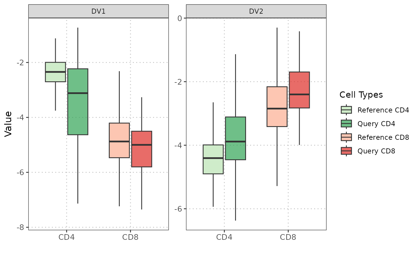
The S3 plot method generates a pairs plot visualization of discriminant vectors, similar to PCA plot visualization. Each panel shows the relationship between two discriminant vectors with customizable display options for lower, diagonal, and upper panels. The visualization allows for comprehensive examination of the discriminant space structure and cell type separability.

References

Fisher, R. A. (1936). "The Use of Multiple Measurements in Taxonomic Problems". *Annals of Eugenics*. 7 (2): 179–188. doi:10.1111/j.1469-1809.1936.tb02137.x.
Hastie, T., Tibshirani, R., & Friedman, J. (2009). *The Elements of Statistical Learning: Data Mining, Inference, and Prediction*. Springer. Chapter 4: Linear Methods for Classification.
Ledoit, O., & Wolf, M. (2004). "A well-conditioned estimator for large-dimensional covariance matrices". *Journal of Multivariate Analysis*. 88 (2): 365–411. doi:10.1016/S0047-259X(03)00096-4.
De Maesschalck, R., Jouan-Rimbaud, D., & Massart, D. L. (2000). "The Mahalanobis distance". *Chemometrics and Intelligent Laboratory Systems*. 50 (1): 1–18. doi:10.1016/S0169-7439(99)00047-7.
Breiman, L. (2001). "Random Forests". *Machine Learning*. 45 (1): 5–32. doi:10.1023/A:1010933404324.

Author

Anthony Christidis, anthony-alexander_christidis@hms.harvard.edu

Examples

# Load data
data("reference_data")
data("query_data")

# Compute discriminant space using unified model across all cell types
disc_output <- calculateDiscriminantSpace(reference_data = reference_data,
                                          query_data = query_data,
                                          query_cell_type_col = "SingleR_annotation",
                                          ref_cell_type_col = "expert_annotation",
                                          n_tree = 500,
                                          n_top = 50,
                                          eigen_threshold  = 1e-1,
                                          calculate_metrics = FALSE,
                                          alpha = 0.01)

# Generate scatter and boxplot
plot(disc_output, plot_type = "scatterplot")
#> Picking joint bandwidth of 0.113
#> Picking joint bandwidth of 0.125
#> Picking joint bandwidth of 0.162

plot(disc_output, cell_types = c("CD4", "CD8"), plot_type = "boxplot")
#> Picking joint bandwidth of 0.0378
#> Picking joint bandwidth of 0.085
#> Picking joint bandwidth of 0.221


# Check comparison
table(Expert_Annotation = query_data$expert_annotation,
      SingleR = query_data$SingleR_annotation)
#>                  SingleR
#> Expert_Annotation B_and_plasma CD4 CD8 Myeloid
#>      B_and_plasma           98   3   1       0
#>      CD4                     0 133   5       0
#>      CD8                     0  44 186       0
#>      Myeloid                 0   0   0      33