Compare Canonical Correlation Analysis (CCA) between Query and Reference Data
Source:R/compareCCA.R, R/plot.compareCCAObject.R
compareCCA.RdThis function performs Canonical Correlation Analysis (CCA) between two datasets (query and reference) after performing PCA on each dataset. It projects the query data onto the PCA space of the reference data and then computes the cosine similarity of the canonical correlation vectors between the two datasets.
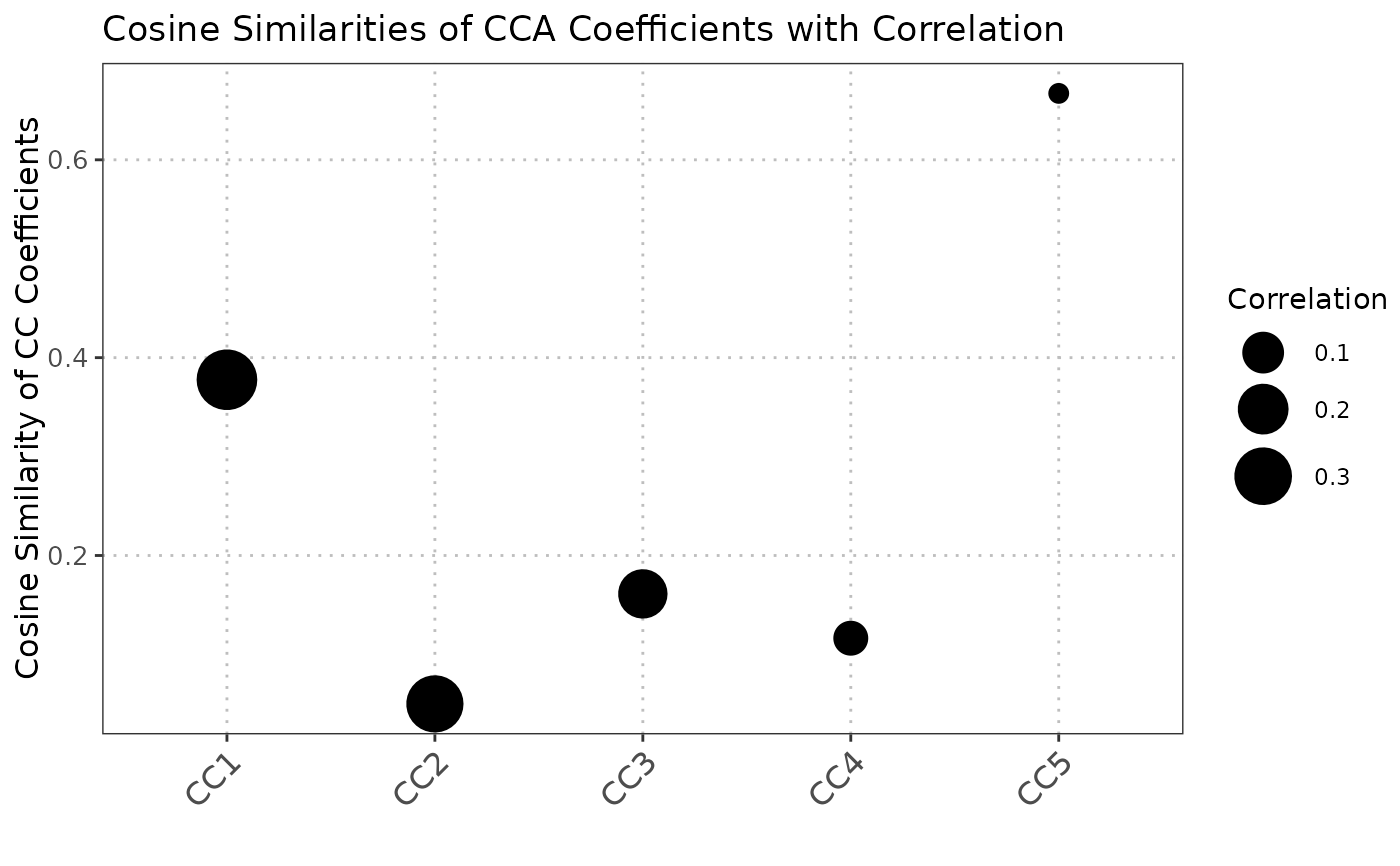
The S3 plot method generates a visualization of the output from the `compareCCA` function. The plot shows the cosine similarities of canonical correlation analysis (CCA) coefficients, with point sizes representing the correlations.
compareCCA(
  query_data,
  reference_data,
  query_cell_type_col,
  ref_cell_type_col,
  pc_subset = 1:5,
  assay_name = "logcounts"
)

# S3 method for class 'compareCCAObject'
plot(x, ...)
Arguments
- query_data
A
SingleCellExperimentobject containing numeric expression matrix for the query cells.- reference_data
A
SingleCellExperimentobject containing numeric expression matrix for the reference cells.- query_cell_type_col
The column name in the
colDataofquery_datathat identifies the cell types.- ref_cell_type_col
The column name in the
colDataofreference_datathat identifies the cell types.- pc_subset
A numeric vector specifying the subset of principal components (PCs) to compare. Default is the first five PCs.
- assay_name
Name of the assay on which to perform computations. Default is "logcounts".
- x
A list containing the output from the
compareCCAfunction. This list should includecosine_similarityandcorrelations.- ...
Additional arguments passed to the plotting function.
Value
A list containing the following elements:
- coef_ref
Canonical coefficients for the reference dataset.
- coef_query
Canonical coefficients for the query dataset.
- cosine_similarity
Cosine similarity values for the canonical variables.
- correlations
Canonical correlations between the reference and query datasets.
The S3 plot method returns a ggplot object representing the scatter plot of cosine similarities of CCA coefficients and correlations.
Details
The function performs the following steps: 1. Projects the query data onto the PCA space of the reference data using the specified number of principal components. 2. Downsamples the datasets to ensure an equal number of rows for CCA. 3. Performs CCA on the projected datasets. 4. Computes the cosine similarity between the canonical correlation vectors and extracts the canonical correlations.
The cosine similarity provides a measure of alignment between the canonical correlation vectors of the two datasets. Higher values indicate greater similarity.
The S3 plot method converts the input list into a data frame suitable for plotting with ggplot2.
Each point in the scatter plot represents the cosine similarity of CCA coefficients, with the size of the point
indicating the correlation.
References
Hotelling, H. (1936). "Relations between two sets of variates". *Biometrika*, 28(3/4), 321-377. doi:10.2307/2333955.
See also
plot.compareCCAObject
compareCCA
Examples
# Load libraries
library(scran)
#> Loading required package: SingleCellExperiment
#> Loading required package: SummarizedExperiment
#> Loading required package: MatrixGenerics
#> Loading required package: matrixStats
#>
#> Attaching package: ‘MatrixGenerics’
#> The following objects are masked from ‘package:matrixStats’:
#>
#>     colAlls, colAnyNAs, colAnys, colAvgsPerRowSet, colCollapse,
#>     colCounts, colCummaxs, colCummins, colCumprods, colCumsums,
#>     colDiffs, colIQRDiffs, colIQRs, colLogSumExps, colMadDiffs,
#>     colMads, colMaxs, colMeans2, colMedians, colMins, colOrderStats,
#>     colProds, colQuantiles, colRanges, colRanks, colSdDiffs, colSds,
#>     colSums2, colTabulates, colVarDiffs, colVars, colWeightedMads,
#>     colWeightedMeans, colWeightedMedians, colWeightedSds,
#>     colWeightedVars, rowAlls, rowAnyNAs, rowAnys, rowAvgsPerColSet,
#>     rowCollapse, rowCounts, rowCummaxs, rowCummins, rowCumprods,
#>     rowCumsums, rowDiffs, rowIQRDiffs, rowIQRs, rowLogSumExps,
#>     rowMadDiffs, rowMads, rowMaxs, rowMeans2, rowMedians, rowMins,
#>     rowOrderStats, rowProds, rowQuantiles, rowRanges, rowRanks,
#>     rowSdDiffs, rowSds, rowSums2, rowTabulates, rowVarDiffs, rowVars,
#>     rowWeightedMads, rowWeightedMeans, rowWeightedMedians,
#>     rowWeightedSds, rowWeightedVars
#> Loading required package: GenomicRanges
#> Loading required package: stats4
#> Loading required package: BiocGenerics
#>
#> Attaching package: ‘BiocGenerics’
#> The following objects are masked from ‘package:stats’:
#>
#>     IQR, mad, sd, var, xtabs
#> The following objects are masked from ‘package:base’:
#>
#>     Filter, Find, Map, Position, Reduce, anyDuplicated, aperm, append,
#>     as.data.frame, basename, cbind, colnames, dirname, do.call,
#>     duplicated, eval, evalq, get, grep, grepl, intersect, is.unsorted,
#>     lapply, mapply, match, mget, order, paste, pmax, pmax.int, pmin,
#>     pmin.int, rank, rbind, rownames, sapply, saveRDS, setdiff, table,
#>     tapply, union, unique, unsplit, which.max, which.min
#> Loading required package: S4Vectors
#>
#> Attaching package: ‘S4Vectors’
#> The following object is masked from ‘package:utils’:
#>
#>     findMatches
#> The following objects are masked from ‘package:base’:
#>
#>     I, expand.grid, unname
#> Loading required package: IRanges
#> Loading required package: GenomeInfoDb
#> Loading required package: Biobase
#> Welcome to Bioconductor
#>
#>     Vignettes contain introductory material; view with
#>     'browseVignettes()'. To cite Bioconductor, see
#>     'citation("Biobase")', and for packages 'citation("pkgname")'.
#>
#> Attaching package: ‘Biobase’
#> The following object is masked from ‘package:MatrixGenerics’:
#>
#>     rowMedians
#> The following objects are masked from ‘package:matrixStats’:
#>
#>     anyMissing, rowMedians
#> Loading required package: scuttle
library(scater)
#> Loading required package: ggplot2

# Load data
data("reference_data")
data("query_data")

# Extract CD4 cells
ref_data_subset <- reference_data[, which(reference_data$expert_annotation == "CD4")]
query_data_subset <- query_data[, which(query_data$expert_annotation == "CD4")]

# Selecting highly variable genes (can be customized by the user)
ref_top_genes <- getTopHVGs(ref_data_subset, n = 500)
query_top_genes <- getTopHVGs(query_data_subset, n = 500)

# Intersect the gene symbols to obtain common genes
common_genes <- intersect(ref_top_genes, query_top_genes)
ref_data_subset <- ref_data_subset[common_genes,]
query_data_subset <- query_data_subset[common_genes,]

# Run PCA on datasets separately
ref_data_subset <- runPCA(ref_data_subset)
query_data_subset <- runPCA(query_data_subset)

# Compare CCA
cca_comparison <- compareCCA(query_data = query_data_subset,
                             reference_data = ref_data_subset,
                             query_cell_type_col = "expert_annotation",
                             ref_cell_type_col = "expert_annotation",
                             pc_subset = 1:5)

# Visualize output of CCA comparison
plot(cca_comparison)