Plot Regression Results on Principal Components

The S3 plot method generates plots to visualize the results of regression analyses performed on principal components (PCs) against cell types, datasets, or their interactions.

This function performs linear regression of a covariate of interest onto one or more principal components, based on the data in a SingleCellExperiment object.

# S3 method for class 'regressPCObject'
plot(
  x,
  plot_type = c("r_squared", "variance_contribution", "coefficient_heatmap"),
  alpha = 0.05,
  coefficients_include = NULL,
  ...
)

regressPC(
  query_data,
  reference_data = NULL,
  query_cell_type_col,
  ref_cell_type_col = NULL,
  query_batch_col = NULL,
  cell_types = NULL,
  pc_subset = 1:10,
  adjust_method = c("BH", "holm", "hochberg", "hommel", "bonferroni", "BY", "fdr",
    "none"),
  assay_name = "logcounts",
  max_cells = 2500
)

Arguments

x: An object of class regressPCObject containing the output of the regressPC function
plot_type: Type of plot to generate. Available options: "r_squared", "variance_contribution", "coefficient_heatmap"
alpha: Significance threshold for p-values. Default is 0.05.
coefficients_include: Character vector specifying which coefficient types to include in the coefficient heatmap. Options are c("cell_type", "batch", "interaction"). Default is NULL, which includes all available coefficient types. Only applies to plot_type = "coefficient_heatmap".
...: Additional arguments to be passed to the plotting functions.
query_data: A SingleCellExperiment object containing numeric expression matrix for the query cells.
reference_data: A SingleCellExperiment object containing numeric expression matrix for the reference cells. If NULL, the PC scores are regressed against the cell types of the query data.
query_cell_type_col: The column name in the colData of query_data that identifies the cell types.
ref_cell_type_col: The column name in the colData of reference_data that identifies the cell types.
query_batch_col: The column name in the colData of query_data that identifies the batch or sample. If provided, performs interaction analysis with cell types. Default is NULL.
cell_types: A character vector specifying the cell types to include in the analysis. If NULL, all cell types are included.
pc_subset: A numeric vector specifying which principal components to include in the analysis. Default is PC1 to PC10.
adjust_method: A character string specifying the method to adjust the p-values. Options include "BH", "holm", "hochberg", "hommel", "bonferroni", "BY", "fdr", or "none". Default is "BH" (Benjamini-Hochberg).
assay_name: Name of the assay on which to perform computations. Default is "logcounts".
max_cells: Maximum number of cells to retain. If the object has fewer cells, it is returned unchanged. Default is 2500.

Value

The S3 plot method returns a ggplot object representing the specified plot type.

A list containing

summaries of the linear regression models for each specified principal component,
the corresponding R-squared (R2) values,
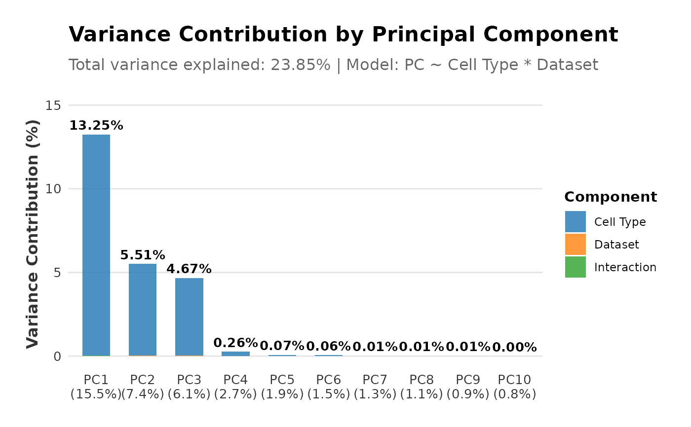
the variance contributions for each principal component, and
the total variance explained.

Details

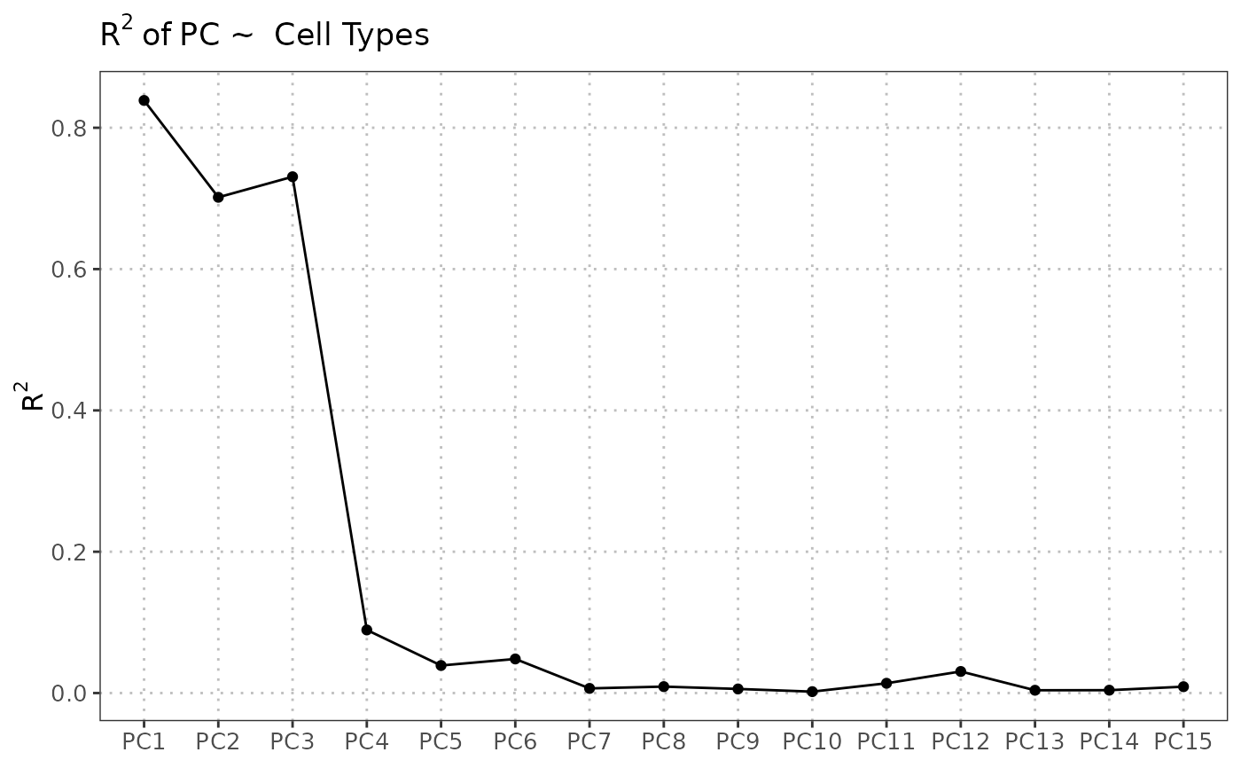
Principal component regression, derived from PCA, can be used to quantify the variance explained by a covariate of interest. Applications for single-cell analysis include quantification of batch effects, assessing clustering homogeneity, and evaluating alignment of query and reference datasets in cell type annotation settings.

The function supports multiple regression scenarios:

Query only, no batch: PC cell_type
Query only, with batch: PC cell_type * batch
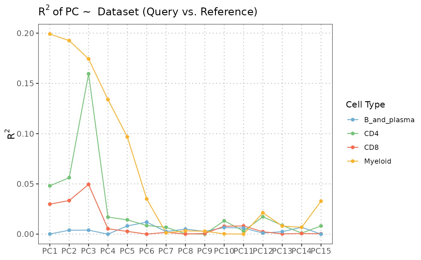
Query + Reference, no batch: PC cell_type * dataset
Query + Reference, with batch: PC cell_type * batch (where batch includes Reference)

When batch information is provided with reference data, batches are labeled as "Reference" for reference data and "Query_BatchName" for query batches, with Reference set as the first factor level for interpretation.

References

Luecken et al. Benchmarking atlas-level data integration in single-cell genomics. Nature Methods, 19:41-50, 2022.

Author

Anthony Christidis, anthony-alexander_christidis@hms.harvard.edu

Examples

# Load data
data("reference_data")
data("query_data")

# Query only analysis
regress_res <- regressPC(query_data = query_data,
                         query_cell_type_col = "expert_annotation",
                         cell_types = c("CD4", "CD8", "B_and_plasma", "Myeloid"),
                         pc_subset = 1:10)
# Visualize results
plot(regress_res, plot_type = "r_squared")

plot(regress_res, plot_type = "variance_contribution")

plot(regress_res, plot_type = "coefficient_heatmap")


# Query + Reference analysis
regress_res <- regressPC(query_data = query_data,
                         reference_data = reference_data,
                         query_cell_type_col = "SingleR_annotation",
                         ref_cell_type_col = "expert_annotation",
                         cell_types = c("CD4", "CD8", "B_and_plasma", "Myeloid"),
                         pc_subset = 1:10)
# Visualize results
plot(regress_res, plot_type = "r_squared")

plot(regress_res, plot_type = "variance_contribution")

plot(regress_res, plot_type = "coefficient_heatmap")