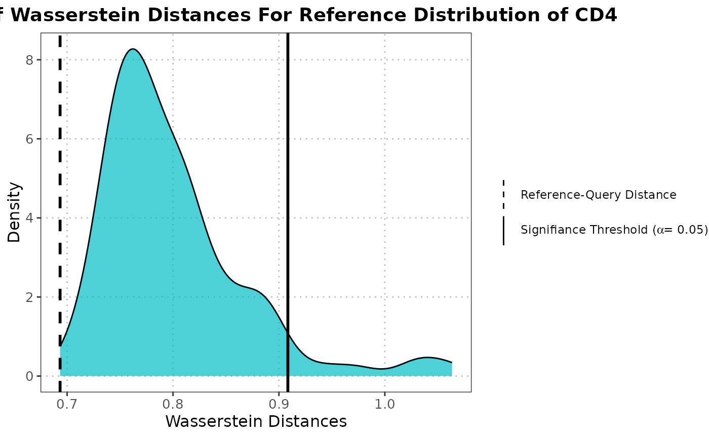
Plot Density of Wasserstein Distances for Null Distribution

This function generates a density plot of Wasserstein distances for the null distribution of a `calculateWassersteinDistanceObject`. Additionally, it overlays lines representing the significance threshold and the reference-query distance.

# S3 method for class 'calculateWassersteinDistanceObject'
plot(x, alpha = 0.05, ...)

Arguments

x

A list object containing the Wasserstein distance results from the calculateWassersteinDistance function.

alpha

A numeric value specifying the significance level for thresholding. Default is 0.05.

...

Additional arguments for future extensions.

Value

A ggplot2 object representing the ridge plots of Wasserstein distances with annotated p-value.

Details

The density plot visualizes the distribution of Wasserstein distances calculated among reference samples, representing the null distribution. A vertical line marks the significance threshold based on the specified alpha. Another line indicates the mean Wasserstein distance between the reference and query datasets.

References

Schuhmacher, D., Bernhard, S., & Book, M. (2019). "A Review of Approximate Transport in Machine Learning". In *Journal of Machine Learning Research* (Vol. 20, No. 117, pp. 1-61).

See also

calculateWassersteinDistance

Author

Anthony Christidis, anthony-alexander_christidis@hms.harvard.edu

Examples

# Load data
data("reference_data")
data("query_data")

# Extract CD4 cells
ref_data_subset <- reference_data[, which(reference_data$expert_annotation == "CD4")]
query_data_subset <- query_data[, which(query_data$expert_annotation == "CD4")]

# Selecting highly variable genes (can be customized by the user)
ref_top_genes <- scran::getTopHVGs(ref_data_subset, n = 500)
query_top_genes <- scran::getTopHVGs(query_data_subset, n = 500)

# Intersect the gene symbols to obtain common genes
common_genes <- intersect(ref_top_genes, query_top_genes)
ref_data_subset <- ref_data_subset[common_genes,]
query_data_subset <- query_data_subset[common_genes,]

# Run PCA on reference data
ref_data_subset <- scater::runPCA(ref_data_subset)

# Compute Wasserstein null distribution using reference data and observed distances with query data
wasserstein_data <- calculateWassersteinDistance(query_data = query_data_subset,
                                                 reference_data = ref_data_subset,
                                                 query_cell_type_col = "expert_annotation",
                                                 ref_cell_type_col = "expert_annotation",
                                                 pc_subset = 1:5,
                                                 n_resamples = 100)
plot(wasserstein_data)