#fname <- file.choose()  # airway_colData.csv
#fnameWorking with summarized experimental data
This section introduces another broadly useful package and data structure, the SummarizedExperiment package and SummarizedExperiment object.

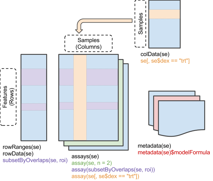
The SummarizedExperiment object has matrix-like properties – it has two dimensions and can be subset by ‘rows’ and ‘columns’. The assay() data of a SummarizedExperiment experiment contains one or more matrix-like objects where rows represent features of interest (e.g., genes), columns represent samples, and elements of the matrix represent results of a genomic assay (e.g., counts of reads overlaps genes in each sample of an bulk RNA-seq differential expression assay.
Object construction
The SummarizedExperiment coordinates assays with (optional) descriptions of rows and columns. We start by reading in a simple data.frame describing 8 samples from an RNASeq experiment looking at dexamethasone treatment across 4 human smooth muscle cell lines; use browseVignettes("airway") for a more complete description of the experiment and data processing. Read the column data in using file.choose() and read.csv().
We want the first column the the data to be treated as row names (sample identifiers) in the data.frame, so read.csv() has an extra argument to indicate this.
colData <- read.csv(fname, row.names = 1)
head(colData)
SampleName cell dex albut Run avgLength Experiment
SRR1039508 GSM1275862 N61311 untrt untrt SRR1039508 126 SRX384345
SRR1039509 GSM1275863 N61311 trt untrt SRR1039509 126 SRX384346
SRR1039512 GSM1275866 N052611 untrt untrt SRR1039512 126 SRX384349
SRR1039513 GSM1275867 N052611 trt untrt SRR1039513 87 SRX384350
SRR1039516 GSM1275870 N080611 untrt untrt SRR1039516 120 SRX384353
SRR1039517 GSM1275871 N080611 trt untrt SRR1039517 126 SRX384354
Sample BioSample
SRR1039508 SRS508568 SAMN02422669
SRR1039509 SRS508567 SAMN02422675
SRR1039512 SRS508571 SAMN02422678
SRR1039513 SRS508572 SAMN02422670
SRR1039516 SRS508575 SAMN02422682
SRR1039517 SRS508576 SAMN02422673The data are from the Short Read Archive, and the row names, SampleName, Run, Experiment, Sampel, and BioSample columns are classifications from the archive. Additional columns include:
cell: the cell line used. There are four cell lines.dex: whether the sample was untreated, or treated with dexamethasone.albut: a second treatment, which we ignoreavgLength: the sample-specific average length of the RNAseq reads estimated in the experiment.
Assay data
Now import the assay data from the file “airway_counts.csv”
fname <- file.choose()  # airway_counts.csv
fname
counts <- read.csv(fname, row.names=1)Although the data are read as a data.frame, all columns are of the same type (integer-valued) and represent the same attribute; the data is really a matrix rather than data.frame, so we coerce to matrix using as.matrix().
counts <- as.matrix(counts)We see the dimensions and first few rows of the counts matrix
dim(counts)[1] 33469 8head(counts) SRR1039508 SRR1039509 SRR1039512 SRR1039513 SRR1039516
ENSG00000000003 679 448 873 408 1138
ENSG00000000419 467 515 621 365 587
ENSG00000000457 260 211 263 164 245
ENSG00000000460 60 55 40 35 78
ENSG00000000938 0 0 2 0 1
ENSG00000000971 3251 3679 6177 4252 6721
SRR1039517 SRR1039520 SRR1039521
ENSG00000000003 1047 770 572
ENSG00000000419 799 417 508
ENSG00000000457 331 233 229
ENSG00000000460 63 76 60
ENSG00000000938 0 0 0
ENSG00000000971 11027 5176 7995It’s interesting to think about what the counts mean – for ENSG00000000003, sample SRR1039508 had 679 reads that overlapped this gene, sample SRR1039509 had 448 reads, etc. Notice that for this gene there seems to be a consistent pattern – within a cell line, the read counts in the untreated group are always larger than the read counts for the treated group. This and other basic observations from ‘looking at’ the data motivate many steps in a rigorous RNASeq differential expression analysis.
Creating a SummarizedExperiment object
There is considerable value in tightly coupling of the column data with the assay data, as it reduces the chances of bookkeeping errors as we work with our data.
Attach the SummarizedExperiment library to our R session.
library("SummarizedExperiment")Use the SummarizedExperiment() function to coordinate the assay and column data; this function uses row and column names to make sure the correct assay columns are described by the correct column data rows.
se <- SummarizedExperiment(assay = list(count=counts), colData = colData)
se
class: SummarizedExperiment
dim: 33469 8
metadata(0):
assays(1): count
rownames(33469): ENSG00000000003 ENSG00000000419 ... ENSG00000273492
ENSG00000273493
rowData names(0):
colnames(8): SRR1039508 SRR1039509 ... SRR1039520 SRR1039521
colData names(9): SampleName cell ... Sample BioSampleIt is straight-forward to use subset() on SummarizedExperiment to create subsets of the data in a coordinated way. Remember that a SummarizedExperiment is conceptually two-dimensional (matrix-like), and in the example below we are subsetting on the second dimension.
subset(se, , dex == "trt")class: SummarizedExperiment
dim: 33469 4
metadata(0):
assays(1): count
rownames(33469): ENSG00000000003 ENSG00000000419 ... ENSG00000273492
ENSG00000273493
rowData names(0):
colnames(4): SRR1039509 SRR1039513 SRR1039517 SRR1039521
colData names(9): SampleName cell ... Sample BioSampleThere are also accessors that extract data from the SummarizedExperiment. For instance, we can use assay() to extract the count matrix, and colSums() to calculate the library size (total number of reads overlapping genes in each sample).
colSums(assay(se))SRR1039508 SRR1039509 SRR1039512 SRR1039513 SRR1039516 SRR1039517 SRR1039520
20637971 18809481 25348649 15163415 24448408 30818215 19126151
SRR1039521
21164133 Note that library sizes differ by a factor of 2 from largest to smallest; how would this influence the interpretation of counts in individual cells of the assay data?
It might be useful to remember important computations in a way that is robust, e.g.,
se$lib.size <- colSums(assay(se))
colData(se)
DataFrame with 8 rows and 10 columns
SampleName cell dex albut Run
<character> <character> <character> <character> <character>
SRR1039508 GSM1275862 N61311 untrt untrt SRR1039508
SRR1039509 GSM1275863 N61311 trt untrt SRR1039509
SRR1039512 GSM1275866 N052611 untrt untrt SRR1039512
SRR1039513 GSM1275867 N052611 trt untrt SRR1039513
SRR1039516 GSM1275870 N080611 untrt untrt SRR1039516
SRR1039517 GSM1275871 N080611 trt untrt SRR1039517
SRR1039520 GSM1275874 N061011 untrt untrt SRR1039520
SRR1039521 GSM1275875 N061011 trt untrt SRR1039521
avgLength Experiment Sample BioSample lib.size
<integer> <character> <character> <character> <numeric>
SRR1039508 126 SRX384345 SRS508568 SAMN02422669 20637971
SRR1039509 126 SRX384346 SRS508567 SAMN02422675 18809481
SRR1039512 126 SRX384349 SRS508571 SAMN02422678 25348649
SRR1039513 87 SRX384350 SRS508572 SAMN02422670 15163415
SRR1039516 120 SRX384353 SRS508575 SAMN02422682 24448408
SRR1039517 126 SRX384354 SRS508576 SAMN02422673 30818215
SRR1039520 101 SRX384357 SRS508579 SAMN02422683 19126151
SRR1039521 98 SRX384358 SRS508580 SAMN02422677 21164133Exercises
This lesson was adapted from materials created by Ludwig Geistlinger