Calculation of Distances Between Specific Cells and Cell Populations
Anthony Christidis
Core for Computational Biomedicine, Harvard Medical SchoolAndrew Ghazi
Core for Computational Biomedicine, Harvard Medical SchoolSmriti Chawla
Core for Computational Biomedicine, Harvard Medical SchoolNitesh Turaga
Core for Computational Biomedicine, Harvard Medical SchoolLudwig Geistlinger
Core for Computational Biomedicine, Harvard Medical SchoolRobert Gentleman
Core for Computational Biomedicine, Harvard Medical SchoolSource:
vignettes/CellDistancesDiagnostics.Rmd
CellDistancesDiagnostics.RmdIntroduction
This vignette demonstrates the use of two functions,
calculateCellDistances() and
calculateCellDistancesSimilarity(), to analyze the
distances between cells in query and reference datasets and to measure
the similarity of density distributions. These functions are useful for
investigating how cells in different datasets relate to each other,
particularly in the context of identifying anomalies and understanding
distribution overlaps.
Datasets
In the context of the scDiagnostics package, the
following datasets illustrate the application of these tools:
reference_data: A curated and processed dataset containing expert-assigned cell type annotations. This dataset serves as a reference for comparison and can be used alone to detect anomalies within the reference annotations.query_data: A dataset that also includes expert-assigned cell type annotations, but additionally features annotations generated by the SingleR package. This allows for the comparison of expert annotations with those produced by an automated method to detect inconsistencies or anomalies.
# Load library
library(scDiagnostics)

# Load datasets
data("reference_data")
data("query_data")

# Set seed for reproducibility
set.seed(0)
Computing Cell Distances
The calculateCellDistances() function calculates
Euclidean distances between cells within the reference dataset and
between query cells and reference cells. This helps in understanding how
closely related cells are within and across datasets based on their
principal component (PC) scores.
Function Usage
# Compute cell distances
distance_data <- calculateCellDistances(
    query_data = query_data,
    reference_data = reference_data,
    query_cell_type_col = "SingleR_annotation",
    ref_cell_type_col = "expert_annotation",
    pc_subset = 1:10
)
In the code above:
-
query_dataand reference_data: These are SingleCellExperiment objects containing the respective datasets for analysis. -
query_cell_type_coland ref_cell_type_col: These arguments specify the columns in thecolDataof each dataset that contain cell type annotations. -
pc_subset: Specifies which principal components (1 to 10) are used to compute distances. PCA is applied for dimensionality reduction before calculating distances.
Output
The output distance_data is a list where each entry
contains:
-
ref_distances: Pairwise distances within the reference dataset for each cell type. -
query_to_ref_distances: Distances from each query cell to all reference cells for each cell type.
Example Workflow
In the example workflow, the first step involves plotting the distributions of cell distances for selected query cells against various reference cell populations. This involves visualizing both the distances between the query cells and the reference cells as well as the distances among the reference cells themselves. For each cell type, such as CD4 and CD8, these plots illustrate how the selected query cells compare in terms of their proximity to different reference populations.
# Identify top 6 anomalies for CD4 cells
cd4_anomalies <- detectAnomaly(
  reference_data = reference_data,
  query_data = query_data,
  query_cell_type_col = "SingleR_annotation",
  ref_cell_type_col = "expert_annotation",
  pc_subset = 1:10,
  n_tree = 500,
  anomaly_treshold = 0.5)

# Top 6 CD4 anomalies
cd4_top6_anomalies <- names(sort(cd4_anomalies$CD4$query_anomaly_scores, decreasing = TRUE)[1:6])

# Plot distances for CD4 and CD8 cells
plot(distance_data, ref_cell_type = "CD4", cell_names = cd4_top6_anomalies)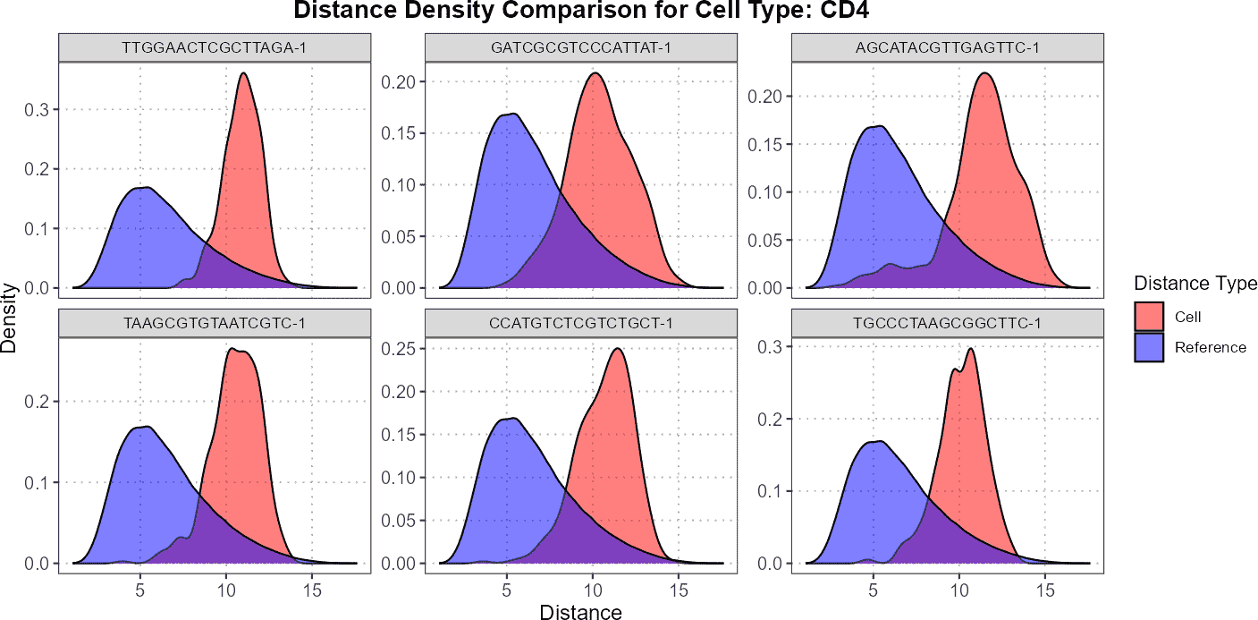
For CD4 cells, you might observe that the query cells are located much further away from the reference cells, indicating a significant divergence in their density distributions. This suggests that the CD4 query cells are less similar to the CD4 reference cells, showing greater variation or potential anomalies.
In contrast, for CD8 cells, the plots might reveal more overlap between the density distributions of query cells and reference cells. This overlap indicates that the CD8 query cells are more similar to the CD8 reference cells, suggesting better alignment or less divergence between their densities. Such insights are crucial for understanding how closely the query cells match with reference populations and can help in identifying cell types with notable differences or similarities.
# Plot distances for CD8 cells
plot(distance_data, ref_cell_type = "CD8", cell_names = cd4_top6_anomalies)
Calculating Similarity Measures
The calculateCellDistancesSimilarity() function measures
how similar the density distributions of query cells are to those in the
reference dataset. It computes Bhattacharyya
coefficients and Hellinger distances, which
quantify the overlap between the distributions.
The Bhattacharyya coefficient and Hellinger distance are two measures used to quantify the similarity between probability distributions. The Bhattacharyya coefficient ranges from 0 to 1, where a value closer to 1 indicates higher similarity between distributions, while a value closer to 0 suggests greater dissimilarity. The Hellinger distance, also ranging from 0 to 1, reflects the divergence between distributions, with lower values indicating greater similarity and higher values showing more distinct distributions. In the context of comparing query cells to reference cells, a high Bhattacharyya coefficient and a low Hellinger distance both suggest that the query cells have density profiles similar to those in the reference dataset, which can be desirable depending on the experimental objectives.
# Compute similarity measures for top 6 CD4 anomalies
overlap_measures <- calculateCellDistancesSimilarity(
  query_data = query_data,
  reference_data = reference_data,
  cell_names = cd4_top6_anomalies,
  query_cell_type_col = "SingleR_annotation",
  ref_cell_type_col = "expert_annotation",
  pc_subset = 1:10)
overlap_measures
#> $bhattacharyya_coef
#>                 Cell       CD4       CD8 B_and_plasma   Myeloid
#> 1 TTGGAACTCGCTTAGA-1 0.4664148 0.9678914    0.3587941 0.2574115
#> 2 GATCGCGTCCCATTAT-1 0.6695226 0.9709480    0.3327168 0.2051765
#> 3 AGCATACGTTGAGTTC-1 0.6526016 0.9609405    0.3085990 0.2102890
#> 4 TAAGCGTGTAATCGTC-1 0.6049953 0.9677820    0.3331004 0.1622547
#> 5 CCATGTCTCGTCTGCT-1 0.6158507 0.9812964    0.3421234 0.2000697
#> 6 TGCCCTAAGCGGCTTC-1 0.6184935 0.9558004    0.3118239 0.1380546
#>
#> $hellinger_dist
#>                 Cell       CD4       CD8 B_and_plasma   Myeloid
#> 1 TTGGAACTCGCTTAGA-1 0.7304692 0.1791887    0.8007534 0.8617357
#> 2 GATCGCGTCCCATTAT-1 0.5748716 0.1704463    0.8168741 0.8915288
#> 3 AGCATACGTTGAGTTC-1 0.5894051 0.1976348    0.8315053 0.8886569
#> 4 TAAGCGTGTAATCGTC-1 0.6284940 0.1794938    0.8166392 0.9152843
#> 5 CCATGTCTCGTCTGCT-1 0.6197978 0.1367610    0.8110959 0.8943882
#> 6 TGCCCTAAGCGGCTTC-1 0.6176621 0.2102369    0.8295638 0.9284102
Conclusion
This vignette illustrates how to leverage the
calculateCellDistances() and
calculateCellDistancesSimilarity() functions to analyze
cell distances and distribution similarities in single-cell datasets. By
calculating Euclidean distances between cells within and across
datasets, you gain insights into how closely related cells are in the
PCA-reduced space. The subsequent step of computing similarity measures,
such as Bhattacharyya coefficients and Hellinger distances, allows for a
deeper understanding of how similar the density distributions of query
cells are to those in the reference dataset.
R Session Info
R version 4.4.1 (2024-06-14)
Platform: x86_64-pc-linux-gnu
Running under: Ubuntu 22.04.5 LTS

Matrix products: default
BLAS:   /usr/lib/x86_64-linux-gnu/openblas-pthread/libblas.so.3
LAPACK: /usr/lib/x86_64-linux-gnu/openblas-pthread/libopenblasp-r0.3.20.so;  LAPACK version 3.10.0

locale:
 [1] LC_CTYPE=C.UTF-8       LC_NUMERIC=C           LC_TIME=C.UTF-8
 [4] LC_COLLATE=C.UTF-8     LC_MONETARY=C.UTF-8    LC_MESSAGES=C.UTF-8
 [7] LC_PAPER=C.UTF-8       LC_NAME=C              LC_ADDRESS=C
[10] LC_TELEPHONE=C         LC_MEASUREMENT=C.UTF-8 LC_IDENTIFICATION=C

time zone: UTC
tzcode source: system (glibc)

attached base packages:
[1] stats     graphics  grDevices utils     datasets  methods   base

other attached packages:
[1] scDiagnostics_1.0.0 BiocStyle_2.32.1

loaded via a namespace (and not attached):
 [1] SummarizedExperiment_1.34.0 gtable_0.3.5
 [3] xfun_0.47                   bslib_0.8.0
 [5] ggplot2_3.5.1               htmlwidgets_1.6.4
 [7] Biobase_2.64.0              lattice_0.22-6
 [9] generics_0.1.3              vctrs_0.6.5
[11] tools_4.4.1                 stats4_4.4.1
[13] parallel_4.4.1              tibble_3.2.1
[15] fansi_1.0.6                 pkgconfig_2.0.3
[17] Matrix_1.7-0                desc_1.4.3
[19] S4Vectors_0.42.1            lifecycle_1.0.4
[21] GenomeInfoDbData_1.2.12     farver_2.1.2
[23] compiler_4.4.1              textshaping_0.4.0
[25] munsell_0.5.1               GenomeInfoDb_1.40.1
[27] htmltools_0.5.8.1           sass_0.4.9
[29] yaml_2.3.10                 pkgdown_2.1.1
[31] pillar_1.9.0                crayon_1.5.3
[33] jquerylib_0.1.4             SingleCellExperiment_1.26.0
[35] DelayedArray_0.30.1         cachem_1.1.0
[37] abind_1.4-8                 tidyselect_1.2.1
[39] digest_0.6.37               dplyr_1.1.4
[41] bookdown_0.40               labeling_0.4.3
[43] fastmap_1.2.0               grid_4.4.1
[45] colorspace_2.1-1            cli_3.6.3
[47] SparseArray_1.4.8           magrittr_2.0.3
[49] S4Arrays_1.4.1              utf8_1.2.4
[51] withr_3.0.1                 UCSC.utils_1.0.0
[53] scales_1.3.0                rmarkdown_2.28
[55] XVector_0.44.0              httr_1.4.7
[57] matrixStats_1.4.1           ragg_1.3.3
[59] isotree_0.6.1-1             evaluate_1.0.0
[61] knitr_1.48                  GenomicRanges_1.56.1
[63] IRanges_2.38.1              rlang_1.1.4
[65] Rcpp_1.0.13                 glue_1.7.0
[67] BiocManager_1.30.25         BiocGenerics_0.50.0
[69] jsonlite_1.8.9              R6_2.5.1
[71] MatrixGenerics_1.16.0       systemfonts_1.1.0
[73] fs_1.6.4                    zlibbioc_1.50.0