Statistical Measures to Assess Dataset Alignment
Anthony Christidis
Core for Computational Biomedicine, Harvard Medical SchoolAndrew Ghazi
Core for Computational Biomedicine, Harvard Medical SchoolSmriti Chawla
Core for Computational Biomedicine, Harvard Medical SchoolNitesh Turaga
Core for Computational Biomedicine, Harvard Medical SchoolLudwig Geistlinger
Core for Computational Biomedicine, Harvard Medical SchoolRobert Gentleman
Core for Computational Biomedicine, Harvard Medical SchoolSource:
vignettes/StatisticalMeasures.Rmd
StatisticalMeasures.RmdIntroduction
In single-cell transcriptomics, it is essential to rigorously analyze and interpret the complex data generated from high-throughput experiments. This vignette introduces several key functions that facilitate advanced statistical analysis and data integration within the context of single-cell experiments. Each function serves a specific purpose, aiding in the comprehensive assessment of single-cell data and its associated covariates.
calculateCramerPValue(): This function computes the Cramér’s V statistic, which measures the strength of association between categorical variables. Cramér’s V is particularly useful for quantifying the association strength in contingency tables, providing insight into how strongly different cell types or conditions are related.calculateHotellingPValue(): This function performs Hotelling’s T-squared test, a multivariate statistical test used to assess the differences between two groups of observations. It is useful for comparing the mean vectors of multiple variables and is commonly employed in single-cell data to evaluate group differences in principal component space.calculateNearestNeighborProbabilities(): This function calculates the probability of nearest neighbor assignments in a high-dimensional space. It is used to evaluate the likelihood of a cell belonging to a specific cluster based on its proximity to neighboring cells. This function helps in assessing clustering quality and the robustness of cell type assignments.calculateAveragePairwiseCorrelation(): This function computes the average pairwise correlation between variables or features across cells. It provides an overview of the relationships between different markers or genes, helping to identify correlated features and understand their interactions within the dataset.regressPC(): This function performs linear regression of a covariate of interest onto one or more principal components derived from single-cell data. This analysis helps quantify the variance explained by the covariate and is useful for tasks such as assessing batch effects, clustering homogeneity, and alignment of query and reference datasets.
Together, these functions provide a reliable toolkit for analyzing and interpreting single-cell data, allowing researchers to gain deeper insights into the underlying biological processes and the relationships between different variables and cell types. The following sections of this vignette will guide you through the usage and application of each function, illustrating their role in comprehensive data analysis.
Preliminaries
In the context of the scDiagnostics package, this
vignette demonstrates how to leverage five key functions to evaluate
cell type annotations across two distinct datasets:
reference_data: This dataset provides expert-curated cell type annotations, serving as a gold standard for evaluating the quality of cell type annotations. It acts as a benchmark to assess and detect anomalies or inconsistencies in cell type classification.query_data: This dataset contains cell type annotations from both expert assessments and those generated by the SingleR package. By comparing these annotations with the reference dataset, you can identify discrepancies between manual and automated annotations. This comparison helps in pinpointing inconsistencies and areas that may require further investigation or refinement.
# Load library
library(scDiagnostics)

# Load datasets
data("reference_data")
data("query_data")

# Set seed for reproducibility
set.seed(0)
calculateCramerPValue()
The calculateCramerPValue function is designed to perform the Cramer test for comparing multivariate empirical cumulative distribution functions (ECDFs) between two samples in single-cell data. This test is particularly useful for assessing whether the distributions of principal components (PCs) differ significantly between the reference and query datasets for specific cell types.
To use this function, you first need to provide two key inputs:
reference_data and query_data, both of which
should be SingleCellExperiment
objects containing numeric expression matrices. If
query_data is not supplied, the function will only use the
reference_data. You should also specify the column names
for cell type annotations in both datasets via
ref_cell_type_col and query_cell_type_col. If
cell_types is not provided, the function will automatically
include all unique cell types found in the datasets. The
pc_subset parameter allows you to define which principal
components to include in the analysis, with the default being the first
five PCs.
The function performs the following steps: it first projects the data into PCA space, subsets the data according to the specified cell types and principal components, and then applies the Cramer test to compare the ECDFs between the reference and query datasets. The result is a named vector of p-values from the Cramer test for each cell type, which indicates whether there is a significant difference in the distributions of PCs between the two datasets.
Here’s an example of how to use the
calculateCramerPValue() function:
# Perform Cramer test for the specified cell types and principal components
cramer_test <- calculateCramerPValue(
    reference_data = reference_data,
    query_data = query_data,
    ref_cell_type_col = "expert_annotation",
    query_cell_type_col = "SingleR_annotation",
    cell_types = c("CD4", "CD8", "B_and_plasma", "Myeloid"),
    pc_subset = 1:5
)

# Display the Cramer test p-values
print(cramer_test)
#>          CD4          CD8 B_and_plasma      Myeloid
#>    0.0000000    0.0000000    0.1368631    0.4105894
In this example, the function compares the distributions of the first five principal components between the reference and query datasets for cell types such as “CD4”, “CD8”, “B_and_plasma”, and “Myeloid”. The output is a vector of p-values indicating whether the differences in PC distributions are statistically significant.
calculateHotellingPValue()
The calculateHotellingPValue() function is designed to
compute Hotelling’s T-squared test statistic and corresponding p-values
for comparing multivariate means between reference and query datasets in
the context of single-cell RNA-seq data. This statistical test is
particularly useful for assessing whether the mean vectors of principal
components (PCs) differ significantly between the two datasets, which
can be indicative of differences in the cell type distributions.
To use this function, you need to provide two SingleCellExperiment
objects: query_data and reference_data, each
containing numeric expression matrices. You also need to specify the
column names for cell type annotations in both datasets with
query_cell_type_col and ref_cell_type_col. The
cell_types parameter allows you to choose which cell types
to include in the analysis, and if not specified, the function will
automatically include all cell types present in the datasets. The
pc_subset parameter determines which principal components
to consider, with the default being the first five PCs. Additionally,
n_permutation specifies the number of permutations for
calculating p-values, with a default of 500.
The function works by first projecting the data into PCA space and then performing Hotelling’s T-squared test for each specified cell type to compare the means between the reference and query datasets. It uses permutation testing to determine the p-values, indicating whether the observed differences in means are statistically significant. The result is a named numeric vector of p-values for each cell type.
Here is an example of how to use the
calculateHotellingPValue() function:
# Calculate Hotelling's T-squared test p-values
p_values <- calculateHotellingPValue(
    query_data = query_data,
    reference_data = reference_data,
    query_cell_type_col = "SingleR_annotation",
    ref_cell_type_col = "expert_annotation",
    pc_subset = 1:10
)

# Display the p-values rounded to five decimal places
print(round(p_values, 5))
#>          CD4          CD8 B_and_plasma      Myeloid
#>         0.00         0.00         0.12         0.00
In this example, the function calculates p-values for Hotelling’s T-squared test, focusing on the first ten principal components to assess whether the multivariate means differ significantly between the reference and query datasets for each cell type. The p-values indicate the likelihood of observing the differences by chance and help identify significant disparities in cell type distributions.
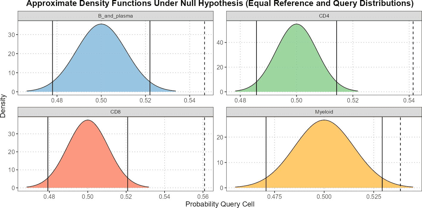
calculateNearestNeighborProbabilities()
In this section, we will explore the
calculateNearestNeighborProbabilities() function, which is
designed to estimate the probability of each query cell belonging to
either the reference or query dataset for each specified cell type. This
function uses nearest neighbor analysis on PCA-reduced data to achieve
this.
The function begins by reducing the dimensionality of both the query and reference datasets using Principal Component Analysis (PCA). It then compares each query cell to its nearest neighbors within the reference dataset. To ensure that sample sizes between datasets are comparable, the function uses data augmentation if necessary.
Here is a detailed explanation of how to use the
calculateNearestNeighborProbabilities() function:
Loading the Data: First, ensure you have the data available in the form of SingleCellExperiment objects for both query and reference datasets.
Function Call: The function
calculateNearestNeighborProbabilities()is called with several parameters including the query and reference datasets, the names of the columns containing cell type annotations, the subset of principal components to use, and the number of nearest neighbors to consider.
# Compute nearest-neighbor probabilities
nn_output <- calculateNearestNeighborProbabilities(
  query_data = query_data,
  reference_data = reference_data,
  query_cell_type_col = "SingleR_annotation",
  ref_cell_type_col = "expert_annotation",
  pc_subset = 1:10,
  n_neighbor = 20
)- Understanding the Output: The output of the function is a list where each element corresponds to a specific cell type. Each element of this list contains:
-
n_neighbor: The number of nearest neighbors considered. -
n_query: The number of cells in the query dataset for that cell type. -
query_prob: The average probability of each query cell belonging to the reference dataset.
-
Plotting the Results: To visualize the results, you
can use the
plotfunction provided for objects of classcalculateNearestNeighborProbabilities.
In summary, the calculateNearestNeighborProbabilities()
function provides a robust method for classifying query cells based on
nearest neighbor analysis in PCA space. This can be particularly useful
for understanding how query cells relate to known reference datasets and
for visualizing these relationships across different cell types.
calculateAveragePairwiseCorrelation()
The calculateAveragePairwiseCorrelation() function is
designed to compute the average pairwise correlations between specified
cell types in single-cell gene expression data. This function operates
on SingleCellExperiment
objects and is ideal for single-cell analysis workflows. It calculates
pairwise correlations between query and reference cells using a
specified correlation method, and then averages these correlations for
each cell type pair. This helps in assessing the similarity between
cells in the reference and query datasets and provides insights into the
reliability of cell type annotations.
To use the calculateAveragePairwiseCorrelation()
function, you need to supply it with two SingleCellExperiment
objects: one for the query cells and one for the reference cells. The
function also requires column names specifying cell type annotations in
both datasets, and optionally a vector of cell types to include in the
analysis. Additionally, you can specify a subset of principal components
to use, or use the raw data directly if pc_subset is set to
NULL. The correlation method can be either “spearman” or
“pearson”.
Here’s an example of how to use this function:
# Compute pairwise correlations between specified cell types
cor_matrix_avg <- calculateAveragePairwiseCorrelation(
  query_data = query_data,
  reference_data = reference_data,
  query_cell_type_col = "SingleR_annotation",
  ref_cell_type_col = "expert_annotation",
  cell_types = c("CD4", "CD8", "B_and_plasma"),
  pc_subset = 1:5,
  correlation_method = "spearman"
)

# Visualize the average pairwise correlation matrix
plot(cor_matrix_avg)
In this example, calculateAveragePairwiseCorrelation()
computes the average pairwise correlations for the cell types “CD4”,
“CD8”, and “B_and_plasma”. This function is particularly useful for
understanding the relationships between different cell types in your
single-cell datasets and evaluating how well cell types in the query
data correspond to those in the reference data.
regressPC()
The regressPC() function performs linear regression of a
covariate of interest onto one or more principal components using data
from a SingleCellExperiment
object. This method helps quantify the variance explained by a
covariate, which can be useful in applications such as quantifying batch
effects, assessing clustering homogeneity, and evaluating alignment
between query and reference datasets in cell type annotation
settings.
The function calculates the R-squared value from the linear regression of the covariate onto each principal component. The variance contribution of the covariate effect per principal component is computed as the product of the variance explained by the principal component and the R-squared value. The total variance explained by the covariate is obtained by summing these contributions across all principal components.
Here is how you can use the regressPC() function:
# Perform regression analysis using only reference data
regress_res <- regressPC(
    reference_data = reference_data,
    ref_cell_type_col = "expert_annotation",
    cell_types = c("CD4", "CD8", "B_and_plasma", "Myeloid"),
    pc_subset = 1:15
)

# Plot results showing R-squared values
plot(regress_res, plot_type = "r_squared")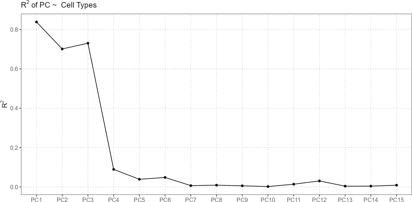
# Plot results showing p-values
plot(regress_res, plot_type = "p-value")
In this example, regressPC() is used to perform
regression analysis on principal components 1 to 15 from the reference
dataset. The results are then visualized using plots showing the
R-squared values and p-values.
If you also have a query dataset and want to compare it with the reference dataset, you can include it in the analysis:
# Perform regression analysis using both reference and query data
regress_res <- regressPC(
    reference_data = reference_data,
    query_data = query_data,
    ref_cell_type_col = "expert_annotation",
    query_cell_type_col = "SingleR_annotation",
    cell_types = c("CD4", "CD8", "B_and_plasma", "Myeloid"),
    pc_subset = 1:15
)

# Plot results showing R-squared values
plot(regress_res, plot_type = "r_squared")
# Plot results showing p-values
plot(regress_res, plot_type = "p-value")
In this case, the function projects the query data onto the principal components of the reference data and performs regression analysis. The results are visualized in the same way, providing insights into how well the principal components from the query data align with those from the reference data.
This function is useful for understanding the impact of different covariates on principal components and for comparing how cell types in different datasets are represented in the principal component space.
Conclusion
The functions introduced in this vignette offer powerful tools for
in-depth analysis and interpretation of single-cell transcriptomics
data. By applying calculateCramerPValue() and
calculateHotellingPValue(), researchers can quantify
associations and differences between categorical variables and
multivariate observations, respectively.
calculateNearestNeighborProbabilities() enhances clustering
analysis by evaluating the likelihood of cell assignments, while
calculateAveragePairwiseCorrelation() reveals relationships
between markers and features. Lastly, regressPC() provides
insights into how principal components relate to covariates, aiding in
the understanding of variance explained by different factors.
Together, these functions enable a comprehensive approach to single-cell data analysis, facilitating the identification of key relationships and enhancing the robustness of conclusions drawn from complex datasets. By leveraging these tools, researchers can advance their understanding of cellular processes and improve the accuracy of data interpretations in single-cell genomics.
R Session Info
R version 4.4.1 (2024-06-14)
Platform: x86_64-pc-linux-gnu
Running under: Ubuntu 22.04.5 LTS

Matrix products: default
BLAS:   /usr/lib/x86_64-linux-gnu/openblas-pthread/libblas.so.3
LAPACK: /usr/lib/x86_64-linux-gnu/openblas-pthread/libopenblasp-r0.3.20.so;  LAPACK version 3.10.0

locale:
 [1] LC_CTYPE=C.UTF-8       LC_NUMERIC=C           LC_TIME=C.UTF-8
 [4] LC_COLLATE=C.UTF-8     LC_MONETARY=C.UTF-8    LC_MESSAGES=C.UTF-8
 [7] LC_PAPER=C.UTF-8       LC_NAME=C              LC_ADDRESS=C
[10] LC_TELEPHONE=C         LC_MEASUREMENT=C.UTF-8 LC_IDENTIFICATION=C

time zone: UTC
tzcode source: system (glibc)

attached base packages:
[1] stats     graphics  grDevices utils     datasets  methods   base

other attached packages:
[1] scDiagnostics_1.0.0 BiocStyle_2.32.1

loaded via a namespace (and not attached):
 [1] SummarizedExperiment_1.34.0 biglm_0.9-3
 [3] gtable_0.3.5                xfun_0.47
 [5] bslib_0.8.0                 ggplot2_3.5.1
 [7] htmlwidgets_1.6.4           Biobase_2.64.0
 [9] lattice_0.22-6              generics_0.1.3
[11] vctrs_0.6.5                 tools_4.4.1
[13] stats4_4.4.1                tibble_3.2.1
[15] fansi_1.0.6                 pkgconfig_2.0.3
[17] Matrix_1.7-0                desc_1.4.3
[19] S4Vectors_0.42.1            lifecycle_1.0.4
[21] GenomeInfoDbData_1.2.12     farver_2.1.2
[23] compiler_4.4.1              textshaping_0.4.0
[25] munsell_0.5.1               GenomeInfoDb_1.40.1
[27] htmltools_0.5.8.1           sass_0.4.9
[29] yaml_2.3.10                 pkgdown_2.1.1
[31] pillar_1.9.0                crayon_1.5.3
[33] jquerylib_0.1.4             MASS_7.3-60.2
[35] SingleCellExperiment_1.26.0 DelayedArray_0.30.1
[37] cachem_1.1.0                boot_1.3-30
[39] abind_1.4-8                 tidyselect_1.2.1
[41] digest_0.6.37               dplyr_1.1.4
[43] bookdown_0.40               labeling_0.4.3
[45] fastmap_1.2.0               grid_4.4.1
[47] colorspace_2.1-1            cli_3.6.3
[49] SparseArray_1.4.8           magrittr_2.0.3
[51] S4Arrays_1.4.1              utf8_1.2.4
[53] withr_3.0.1                 UCSC.utils_1.0.0
[55] scales_1.3.0                rmarkdown_2.28
[57] XVector_0.44.0              httr_1.4.7
[59] matrixStats_1.4.1           ragg_1.3.3
[61] evaluate_1.0.0              knitr_1.48
[63] GenomicRanges_1.56.1        IRanges_2.38.1
[65] rlang_1.1.4                 Rcpp_1.0.13
[67] DBI_1.2.3                   glue_1.7.0
[69] BiocManager_1.30.25         cramer_0.9-4
[71] BiocGenerics_0.50.0         speedglm_0.3-5
[73] jsonlite_1.8.9              R6_2.5.1
[75] MatrixGenerics_1.16.0       systemfonts_1.1.0
[77] fs_1.6.4                    zlibbioc_1.50.0