Density Plot of Wasserstein Distances Under Null Distribution

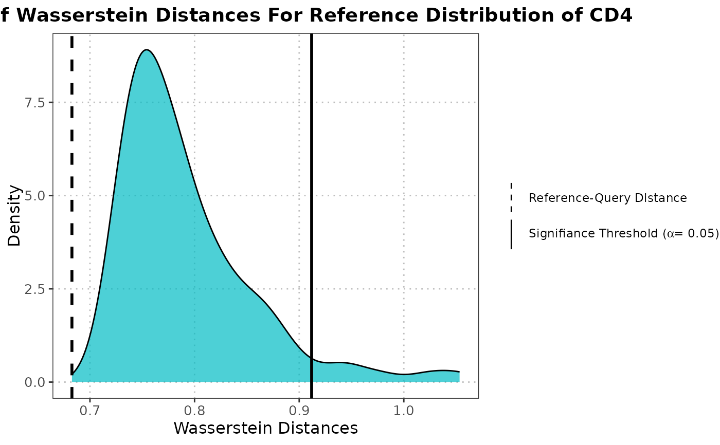
This function generates a density plot of Wasserstein distances under the null hypothesis that the two datasets come from the same distribution. It computes the null distribution of Wasserstein distances and compares it to the distances between reference and query data.

plotWassersteinDistance(
  query_data,
  reference_data,
  ref_cell_type_col,
  query_cell_type_col,
  pc_subset = 1:5,
  n_resamples = 300,
  alpha = 0.05,
  assay_name = "logcounts"
)

Arguments

query_data

A SingleCellExperiment object containing numeric expression matrix for the query cells.

reference_data

A SingleCellExperiment object containing numeric expression matrix for the reference cells.

ref_cell_type_col

The column name in the colData of reference_data that identifies the cell types.

query_cell_type_col

The column name in the colData of query_data that identifies the cell types.

pc_subset

A numeric vector specifying which principal components to include in the plot. Default is 1:5.

n_resamples

An integer specifying the number of resamples to use for generating the null distribution. Default is 300.

alpha

A numeric value specifying the significance level for thresholding. Default is 0.05.

assay_name

Name of the assay on which to perform computations. Default is "logcounts".

Value

A ggplot2 object representing the density plot of Wasserstein distances under the null distribution.

Details

This function first projects the query data onto the PCA space defined by the reference data. It then computes the Wasserstein distances between randomly sampled subsets of the reference data to generate a null distribution. The function also computes the Wasserstein distances between the reference and query data. Finally, it visualizes these distances using a density plot with vertical lines indicating the significance threshold and the reference-query distance.

References

Schuhmacher, D., Bernhard, S., & Book, M. (2019). "A Review of Approximate Transport in Machine Learning". In *Journal of Machine Learning Research* (Vol. 20, No. 117, pp. 1-61).

Author

Anthony Christidis, anthony-alexander_christidis@hms.harvard.edu

Examples

# Load data
data("reference_data")
data("query_data")

# Extract CD4 cells
ref_data_subset <- reference_data[, which(reference_data$expert_annotation == "CD4")]
query_data_subset <- query_data[, which(query_data$expert_annotation == "CD4")]

# Selecting highly variable genes (can be customized by the user)
ref_top_genes <- scran::getTopHVGs(ref_data_subset, n = 500)
query_top_genes <- scran::getTopHVGs(query_data_subset, n = 500)

# Intersect the gene symbols to obtain common genes
common_genes <- intersect(ref_top_genes, query_top_genes)
ref_data_subset <- ref_data_subset[common_genes,]
query_data_subset <- query_data_subset[common_genes,]

# Run PCA on reference data
ref_data_subset <- scater::runPCA(ref_data_subset)

# Compute Wasserstein null distribution using reference data and observed distance with query data
wasserstein_plot <- plotWassersteinDistance(query_data = query_data_subset,
                                            reference_data = ref_data_subset, 
                                            query_cell_type_col = "expert_annotation", 
                                            ref_cell_type_col = "expert_annotation", 
                                            pc_subset = 1:5,
                                            n_resamples = 100,
                                            alpha = 0.05)
wasserstein_plot