Content from Welcome to Python
Last updated on 2023-04-18 | Edit this page
Overview
Questions
- How can I run Python programs?
Objectives
- Launch the JupyterLab server.
- Create a new Python script.
- Create a Jupyter notebook.
- Shutdown the JupyterLab server.
- Understand the difference between a Python script and a Jupyter notebook.
- Create Markdown cells in a notebook.
- Create and run Python cells in a notebook.
Key Points
- Python scripts are plain text files.
- Use the Jupyter Notebook for editing and running Python.
- The Notebook has Command and Edit modes.
- Use the keyboard and mouse to select and edit cells.
- The Notebook will turn Markdown into pretty-printed documentation.
- Markdown does most of what HTML does.
Many software developers will often use an integrated development environment (IDE) or a text editor to create and edit their Python programs which can be executed through the IDE or command line directly. While this is a common approach, we are going to use the [Jupyter Notebook][jupyter] via JupyterLab for the remainder of this workshop.
This has several advantages: * You can easily type, edit, and copy and paste blocks of code. * Tab complete allows you to easily access the names of things you are using and learn more about them. * It allows you to annotate your code with links, different sized text, bullets, etc. to make it more accessible to you and your collaborators. * It allows you to display figures next to the code that produces them to tell a complete story of the analysis.
Each notebook contains one or more cells that contain code, text, or images.
Scripts vs. Notebooks vs. Programs
A notebook, as described above, is a combination of text, figures,
results, and code in a single document. In contrast a script is a file
containing only code (and comments). A python script has the extension
.py, while a python notebook has the extension
.ipynb. Python notebooks are built ontop of Python and are
not considered a part of the Python language, but an extension to it.
Cells in a notebook can be run interactively while a script is run all
at once, typically by calling it at the command line.
A program is a set of machine instructions which are executed together. We can think about both Python scripts and notebooks as being programs. It should be noted, however, that in computer science the terms programming and scripting are defined more formally, and no Python code would be considered a program under these definitions.
Getting Started with JupyterLab
JupyterLab is an application with a web-based user interface from [Project Jupyter][jupyter] that enables one to work with documents and activities such as Jupyter notebooks, text editors, terminals, and even custom components in a flexible, integrated, and extensible manner. JupyterLab requires a reasonably up-to-date browser (ideally a current version of Chrome, Safari, or Firefox); Internet Explorer versions 9 and below are not supported.
JupyterLab is included as part of the Anaconda Python distribution. If you have not already installed the Anaconda Python distribution, see the setup instructions for installation instructions.
Even though JupyterLab is a web-based application, JupyterLab runs locally on your machine and does not require an internet connection. * The JupyterLab server sends messages to your web browser. * The JupyterLab server does the work and the web browser renders the result. * You will type code into the browser and see the result when the web page talks to the JupyterLab server.
JupyterLab? What about Jupyter notebooks?
JupyterLab is the next stage in the evolution of the Jupyter Notebook. If you have prior experience working with Jupyter notebooks, then you will have a good idea of what to expect from JupyterLab.
Experienced users of Jupyter notebooks interested in a more detailed discussion of the similarities and differences between the JupyterLab and Jupyter notebook user interfaces can find more information in the JupyterLab user interface documentation.
Starting JupyterLab
You can start the JupyterLab server through the command line or
through an application called Anaconda Navigator. Anaconda
Navigator is included as part of the Anaconda Python distribution.
macOS - Command Line
To start the JupyterLab server you will need to access the command line through the Terminal. There are two ways to open Terminal on Mac.
- In your Applications folder, open Utilities and double-click on Terminal
- Press Command + spacebar to launch Spotlight.
Type
Terminaland then double-click the search result or hit Enter
After you have launched Terminal, type the command to launch the JupyterLab server.
Windows Users - Command Line
To start the JupyterLab server you will need to access the Anaconda Prompt.
Press Windows Logo Key and search for
Anaconda Prompt, click the result or press enter.
After you have launched the Anaconda Prompt, type the command:
Anaconda Navigator
To start a JupyterLab server from Anaconda Navigator you must first
start
Anaconda Navigator (click for detailed instructions on macOS, Windows,
and Linux). You can search for Anaconda Navigator via Spotlight on
macOS (Command + spacebar), the Windows search
function (Windows Logo Key) or opening a terminal shell and
executing the anaconda-navigator executable from the
command line.
After you have launched Anaconda Navigator, click the
Launch button under JupyterLab. You may need to scroll down
to find it.
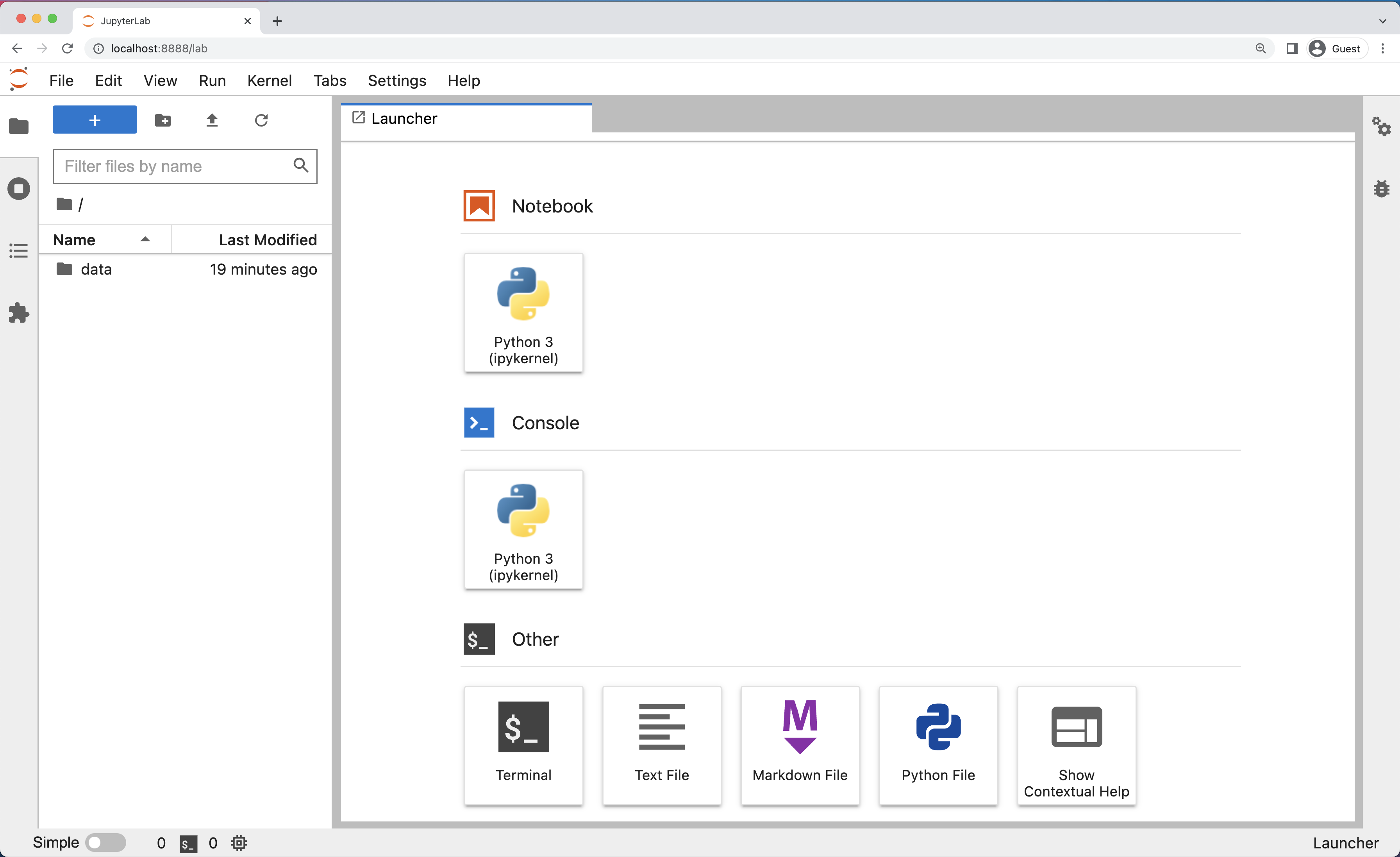
Here is a screenshot of an Anaconda Navigator page similar to the one that should open on either macOS or Windows.

And here is a screenshot of a JupyterLab landing page that should be similar to the one that opens in your default web browser after starting the JupyterLab server on either macOS or Windows.
The JupyterLab Interface
JupyterLab has many features found in traditional integrated development environments (IDEs) but is focused on providing flexible building blocks for interactive, exploratory computing.
The JupyterLab Interface consists of the Menu Bar, a collapsable Left Side Bar, and the Main Work Area which contains tabs of documents and activities.
Menu Bar
The Menu Bar at the top of JupyterLab has the top-level menus that expose various actions available in JupyterLab along with their keyboard shortcuts (where applicable). The following menus are included by default.
- File: Actions related to files and directories such as New, Open, Close, Save, etc. The File menu also includes the Shut Down action used to shutdown the JupyterLab server.
- Edit: Actions related to editing documents and other activities such as Undo, Cut, Copy, Paste, etc.
- View: Actions that alter the appearance of JupyterLab.
- Run: Actions for running code in different activities such as notebooks and code consoles (discussed below).
- Kernel: Actions for managing kernels. Kernels in Jupyter will be explained in more detail below.
- Tabs: A list of the open documents and activities in the main work area.
- Settings: Common JupyterLab settings can be configured using this menu. There is also an Advanced Settings Editor option in the dropdown menu that provides more fine-grained control of JupyterLab settings and configuration options.
- Help: A list of JupyterLab and kernel help links.
Kernels
The JupyterLab docs define kernels as “separate processes started by the server that run your code in different programming languages and environments.” When we open a Jupyter Notebook, that starts a kernel - a process - that is going to run the code. In this lesson, we’ll be using the Jupyter ipython kernel which lets us run Python 3 code interactively.
Using other Jupyter kernels for other programming languages would let us write and execute code in other programming languages in the same JupyterLab interface, like R, Java, Julia, Ruby, JavaScript, Fortran, etc.
A screenshot of the default Menu Bar is provided below.
Left Sidebar
The left sidebar contains a number of commonly used tabs, such as a file browser (showing the contents of the directory where the JupyterLab server was launched), a list of running kernels and terminals, the command palette, and a list of open tabs in the main work area. A screenshot of the default Left Side Bar is provided below.
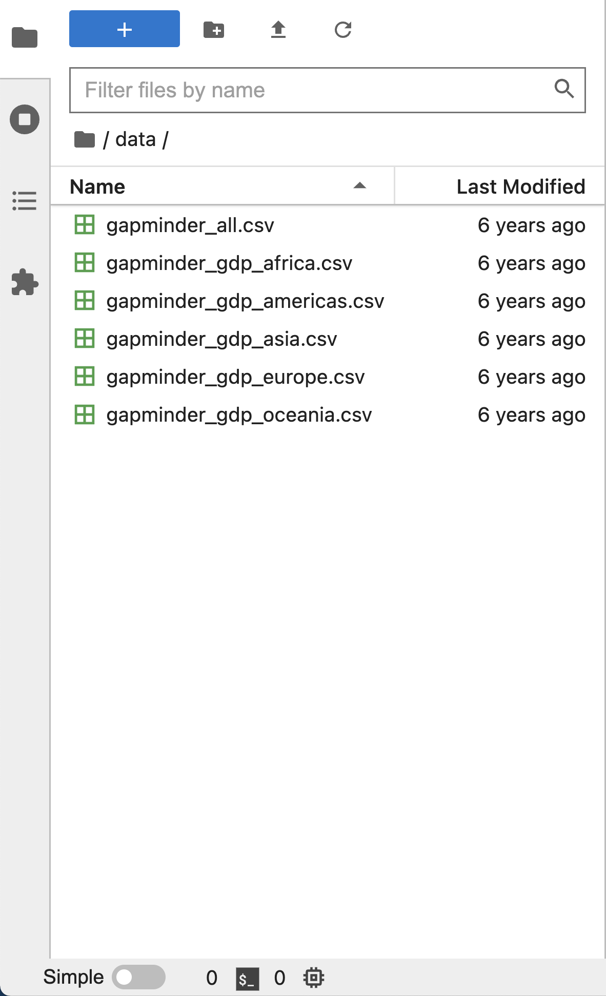
The left sidebar can be collapsed or expanded by selecting “Show Left Sidebar” in the View menu or by clicking on the active sidebar tab.
Main Work Area
The main work area in JupyterLab enables you to arrange documents (notebooks, text files, etc.) and other activities (terminals, code consoles, etc.) into panels of tabs that can be resized or subdivided. A screenshot of the default Main Work Area is provided below.
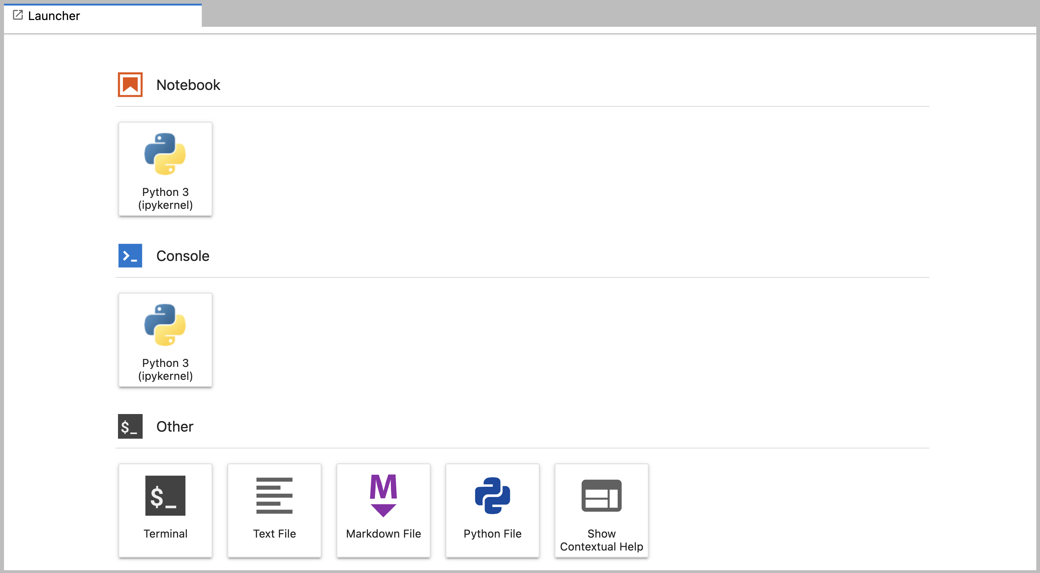
Drag a tab to the center of a tab panel to move the tab to the panel. Subdivide a tab panel by dragging a tab to the left, right, top, or bottom of the panel. The work area has a single current activity. The tab for the current activity is marked with a colored top border (blue by default).
Creating a Python script
- To start writing a new Python program click the Text File icon under
the Other header in the Launcher tab of the Main Work Area.
- You can also create a new plain text file by selecting the New -> Text File from the File menu in the Menu Bar.
- To convert this plain text file to a Python program, select the
Save File As action from the File menu in the Menu Bar
and give your new text file a name that ends with the
.pyextension.- The
.pyextension lets everyone (including the operating system) know that this text file is a Python program. - This is convention, not a requirement.
- The
Creating a Jupyter Notebook
To open a new notebook click the Python 3 icon under the Notebook header in the Launcher tab in the main work area. You can also create a new notebook by selecting New -> Notebook from the File menu in the Menu Bar.
Additional notes on Jupyter notebooks.
- Notebook files have the extension
.ipynbto distinguish them from plain-text Python programs. - Notebooks can be exported as Python scripts that can be run from the command line.
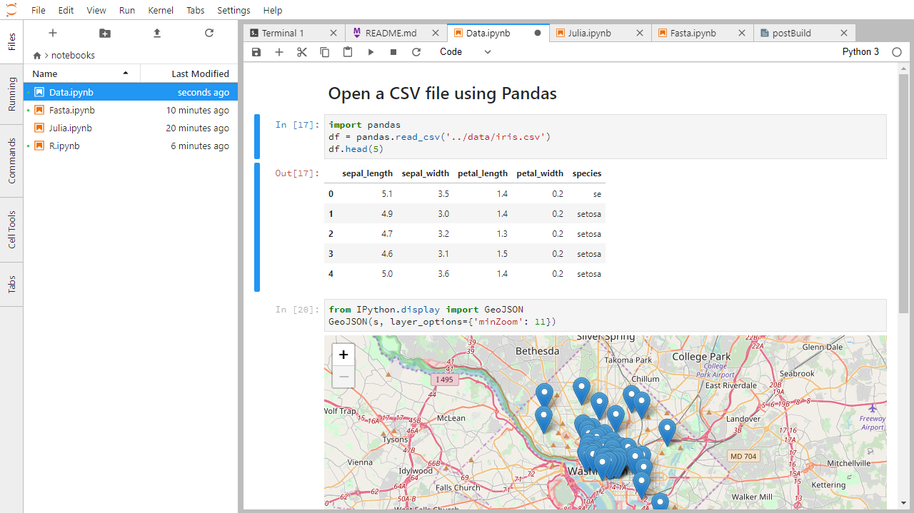
Below is a screenshot of a Jupyter notebook running inside JupyterLab. If you are interested in more details, then see the official notebook documentation.
How It’s Stored
- The notebook file is stored in a format called JSON.
- Just like a webpage, what’s saved looks different from what you see in your browser.
- But this format allows Jupyter to mix source code, text, and images, all in one file.
Arranging Documents into Panels of Tabs
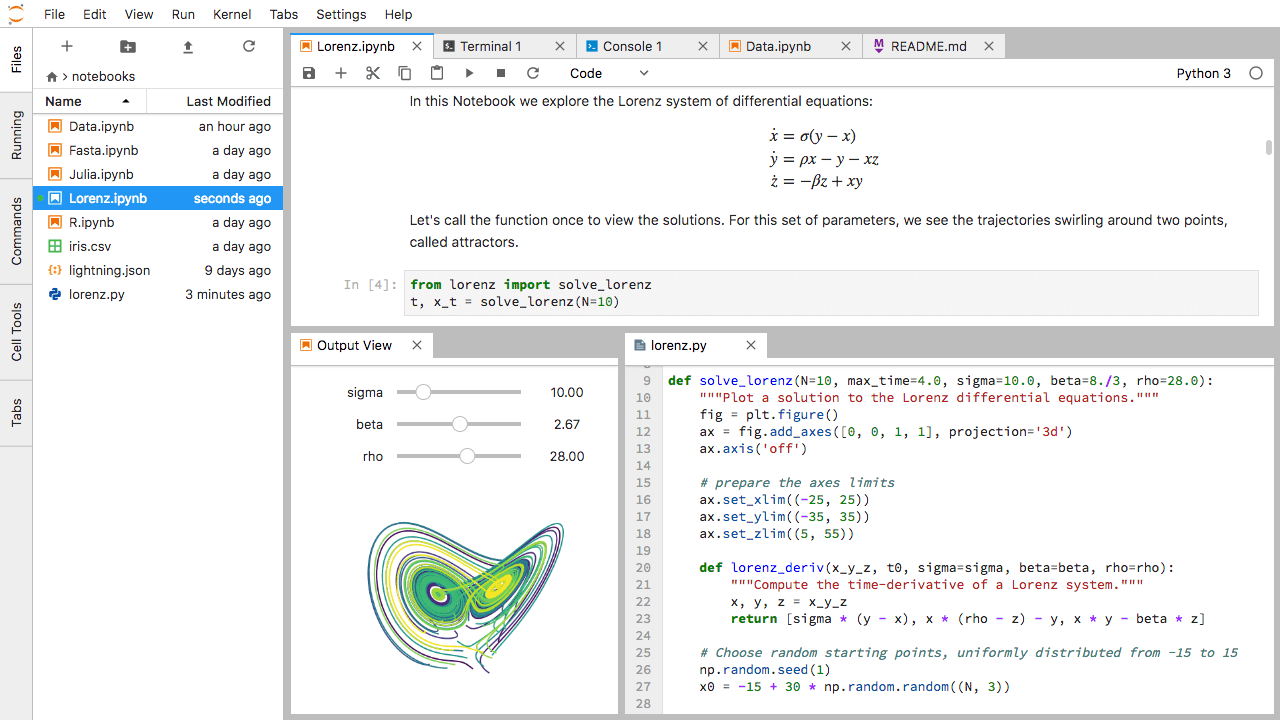
In the JupyterLab Main Work Area you can arrange documents into panels of tabs. Here is an example from the official documentation.
First, create a text file, Python console, and terminal window and arrange them into three panels in the main work area. Next, create a notebook, terminal window, and text file and arrange them into three panels in the main work area. Finally, create your own combination of panels and tabs. What combination of panels and tabs do you think will be most useful for your workflow?
After creating the necessary tabs, you can drag one of the tabs to the center of a panel to move the tab to the panel; next you can subdivide a tab panel by dragging a tab to the left, right, top, or bottom of the panel.
Code vs. Text
Jupyter mixes code and text in different types of blocks, called cells. We often use the term “code” to mean “the source code of software written in a language such as Python”. A “code cell” in a Notebook is a cell that contains software; a “text cell” is one that contains ordinary prose written for human beings.
The Notebook has Command and Edit modes.
- If you press Esc and Return alternately, the outer border of your code cell will change from gray to blue.
- These are the Command (gray) and Edit (blue) modes of your notebook.
- Command mode allows you to edit notebook-level features, and Edit mode changes the content of cells.
- When in Command mode (esc/gray),
- The b key will make a new cell below the currently selected cell.
- The a key will make one above.
- The x key will delete the current cell.
- The z key will undo your last cell operation (which could be a deletion, creation, etc).
- All actions can be done using the menus, but there are lots of keyboard shortcuts to speed things up.
Command Vs. Edit
In the Jupyter notebook page are you currently in Command or Edit
mode?
Switch between the modes. Use the shortcuts to generate a new cell. Use
the shortcuts to delete a cell. Use the shortcuts to undo the last cell
operation you performed.
Command mode has a grey border and Edit mode has a blue border. Use Esc and Return to switch between modes. You need to be in Command mode (Press Esc if your cell is blue). Type b or a. You need to be in Command mode (Press Esc if your cell is blue). Type x. You need to be in Command mode (Press Esc if your cell is blue). Type z.
Use the keyboard and mouse to select and edit cells.
- Pressing the Return key turns the border blue and engages Edit mode, which allows you to type within the cell.
- Because we want to be able to write many lines of code in a single cell, pressing the Return key when in Edit mode (blue) moves the cursor to the next line in the cell just like in a text editor.
- We need some other way to tell the Notebook we want to run what’s in the cell.
- Pressing Shift+Return together will execute the contents of the cell.
- Notice that the Return and Shift keys on the right of the keyboard are right next to each other.
The Notebook will turn Markdown into pretty-printed documentation.
- Notebooks can also render Markdown.
- A simple plain-text format for writing lists, links, and other things that might go into a web page.
- Equivalently, a subset of HTML that looks like what you’d send in an old-fashioned email.
- Turn the current cell into a Markdown cell by entering the Command mode (Esc/gray) and press the M key.
-
In [ ]:will disappear to show it is no longer a code cell and you will be able to write in Markdown. - Turn the current cell into a Code cell by entering the Command mode (Esc/gray) and press the y key.
Markdown does most of what HTML does.
*   Use asterisks
*   to create
* bullet lists.- Use asterisks
- to create
- bullet lists.
1.  Use numbers
1.  to create
1. numbered lists.- Use numbers
- to create
- numbered lists.
*  You can use indents
	*  To create sublists
	*  of the same type
*  Or sublists
	1. Of different
1. types- You can use indents
- To create sublists
- of the same type
- Or sublists
- Of different
- types
Line breaks
don't matter.

But blank lines
create new paragraphs.
Line breaks don’t matter.
But blank lines create new paragraphs.
[Create links](http://software-carpentry.org) with `[...](...)`.
Or use [named links][data_carpentry].

[data_carpentry]: http://datacarpentry.org
Create links with
[...](...). Or use named
links.
Creating Lists in Markdown
Create a nested list in a Markdown cell in a notebook that looks like this:
- Get funding.
- Do work.
- Design experiment.
- Collect data.
- Analyze.
- Write up.
- Publish.
This challenge integrates both the numbered list and bullet list. Note that the bullet list is indented 2 spaces so that it is inline with the items of the numbered list.
1.  Get funding.
1.  Do work.
    *   Design experiment.
    *   Collect data.
    *   Analyze.
1.  Write up.
1. Publish.Python returns the output of the last calculation.
OUTPUT
3Change an Existing Cell from Code to Markdown
What happens if you write some Python in a code cell and then you switch it to a Markdown cell? For example, put the following in a code cell:
And then run it with Shift+Return to be sure that it works as a code cell. Now go back to the cell and use Esc then m to switch the cell to Markdown and “run” it with Shift+Return. What happened and how might this be useful?
Equations
Standard Markdown (such as we’re using for these notes) won’t render equations, but the Notebook will. Create a new Markdown cell and enter the following:
$\sum_{i=1}^{N} 2^{-i} \approx 1$(It’s probably easier to copy and paste.) What does it display? What
do you think the underscore, _, circumflex, ^,
and dollar sign, $, do?
The notebook shows the equation as it would be rendered from LaTeX
equation syntax. The dollar sign, $, is used to tell
Markdown that the text in between is a LaTeX equation. If you’re not
familiar with LaTeX, underscore, _, is used for subscripts
and circumflex, ^, is used for superscripts. A pair of
curly braces, { and }, is used to group text
together so that the statement i=1 becomes the subscript
and N becomes the superscript. Similarly, -i
is in curly braces to make the whole statement the superscript for
2. \sum and \approx are LaTeX
commands for “sum over” and “approximate” symbols.
Closing JupyterLab
- From the Menu Bar select the “File” menu and then choose “Shut Down” at the bottom of the dropdown menu. You will be prompted to confirm that you wish to shutdown the JupyterLab server (don’t forget to save your work!). Click “Shut Down” to shutdown the JupyterLab server.
- To restart the JupyterLab server you will need to re-run the following command from a shell.
$ jupyter labClosing JupyterLab
Practice closing and restarting the JupyterLab server.
Content from Variables in Python
Last updated on 2023-04-18 | Edit this page
Overview
Questions
- How do I run Python code?
- What are variables?
- How do I set variables in Python?
Objectives
- Use the Python console to perform calculations.
- Assign values to variables in Python.
- Reuse variables in Python.
Key Points
- Python is an interpreted programming language, and can be used interactively.
-
Values are assigned to variables
in Python using
=. - You can use
printto output variable values. - Use meaningful variable names.
Variables store values.
- Variables are names for values.
- In Python the
=symbol assigns the value on the right to the name on the left. - The variable is created when a value is assigned to it.
- Here, Python assigns an age to a variable
ageand a name in quotes to a variablefirst_name.
- Variable names
- can only contain letters, digits, and underscore
_(typically used to separate words in long variable names) - cannot start with a digit
- are case sensitive (age, Age and AGE are three different variables)
- can only contain letters, digits, and underscore
- Variable names that start with underscores like
__alistairs_real_agehave a special meaning so we won’t do that until we understand the convention.
Use print to display values.
Callout
A string is the type which stores text in Python. Strings can be thought of as sequences or strings of individual characters (and using the words string this way actually goes back to a printing term in the pre-computer era). We will be learning more about types and strings in other lessons.
- Python has a built-in function called
printthat prints things as text. - Call the function (i.e., tell Python to run it) by using its name.
- Provide values to the function (i.e., the things to print) in parentheses.
- To add a string to the printout, wrap the string in single or double quotes.
- The values passed to the function are called arguments
Single vs. double quotes
In Python, you can use single quotes or double quotes to denote a string, but you need to use the same one for both the beginning and the end.
In Python,
OUTPUT
Ahmed is 42 years old-
printautomatically puts a single space between items to separate them.
In when using Jupyter notebooks, we can also simply write a variable name and its value will be displayed:
OUTPUT
42However, this will not work in other programming environments or when running scripts. We will be displaying variables using both methods throughout this workshop.
Variables must be created before they are used.
- If a variable doesn’t exist yet, or if the name has been mis-spelled, Python reports an error. (Unlike some languages, which “guess” a default value.)
ERROR
---------------------------------------------------------------------------
NameError                                 Traceback (most recent call last)
<ipython-input-1-c1fbb4e96102> in <module>()
----> 1 print(last_name)

NameError: name 'last_name' is not defined- The last line of an error message is usually the most informative.
- We will look at error messages in detail later.
Variables Persist Between Cells
Be aware that it is the order of execution of cells that is important in a Jupyter notebook, not the order in which they appear. Python will remember all the code that was run previously, including any variables you have defined, irrespective of the order in the notebook. Therefore if you define variables lower down the notebook and then (re)run cells further up, those defined further down will still be present. As an example, create two cells with the following content, in this order:
If you execute this in order, the first cell will give an error.
However, if you run the first cell after the second cell it
will print out 1. To prevent confusion, it can be helpful
to use the Kernel -> Restart & Run All
option which clears the interpreter and runs everything from a clean
slate going top to bottom.
Variables can be used in calculations.
- We can use variables in calculations just as if they were values.
- Remember, we assigned the value
42toagea few lines ago.
- Remember, we assigned the value
OUTPUT
Age in three years: 45Python is case-sensitive.
- Python thinks that upper- and lower-case letters are different, so
Nameandnameare different variables. - There are conventions for using upper-case letters at the start of variable names so we will use lower-case letters for now.
Use meaningful variable names.
- Python doesn’t care what you call variables as long as they obey the rules (alphanumeric characters and the underscore).
- Use meaningful variable names to help other people understand what the program does.
- The most important “other person” is your future self.
Try using this python visualization tool to visualize what happens in the code.
OUTPUT
# Command  # Value of x   # Value of y   # Value of swap #
x = 1.0    # 1.0          # not defined  # not defined   #
y = 3.0    # 1.0          # 3.0          # not defined   #
swap = x   # 1.0          # 3.0          # 1.0           #
x = y      # 3.0          # 3.0          # 1.0           #
y = swap   # 3.0          # 1.0          # 1.0           #
These three lines exchange the values in x and
y using the swap variable for temporary
storage. This is a fairly common programming idiom.
Choosing a Name
Which is a better variable name, m, min, or
minutes? Why?
Hint: think about which code you would rather inherit from someone who is leaving the lab:
ts = m * 60 + stot_sec = min * 60 + sectotal_seconds = minutes * 60 + seconds
minutes is better because min might mean
something like “minimum” (and actually is an existing built-in function
in Python that we will cover later).
Content from Basic Types
Last updated on 2023-04-18 | Edit this page
Overview
Questions
- What kinds of data are there in Python?
- How are different data types treated differently?
- How can I identify a variable’s type?
- How can I convert between types?
Objectives
- Explain key differences between integers and floating point numbers.
- Explain key differences between numbers and character strings.
- Use built-in functions to convert between integers, floating point numbers, and strings.
- Subset a string using slicing.
Key Points
- Every value has a type.
- Use the built-in function
typeto find the type of a value. - Types control what operations can be done on values.
- Strings can be added and multiplied.
- Strings have a length (but numbers don’t).
Every value has a type.
- Every value in a program has a specific type.
- Integer (
int): represents positive or negative whole numbers like 3 or -512. - Floating point number (
float): represents real numbers like 3.14159 or -2.5. - Character string (usually called “string”,
str): text.- Written in either single quotes or double quotes (as long as they match).
- The quote marks aren’t printed when the string is displayed.
Use the built-in function type to find the type of a
value.
- Use the built-in function
typeto find out what type a value has. - Works on variables as well.
- But remember: the value has the type — the variable is just a label.
OUTPUT
<class 'int'>OUTPUT
<class 'str'>Types control what operations (or methods) can be performed on a given value.
- A value’s type determines what the program can do to it.
OUTPUT
2OUTPUT
---------------------------------------------------------------------------
TypeError                                 Traceback (most recent call last)
<ipython-input-2-67f5626a1e07> in <module>()
----> 1 print('hello' - 'h')

TypeError: unsupported operand type(s) for -: 'str' and 'str'
Simple and compound types.
We can broadly split different types into two categories in Python: simple types and compound types.
Simple types consist of a single value. In Python, these simple types include:
intfloatboolNoneType
Compound types contain multiple values. Compound types include:
strlistdictionarytupleset
In this lesson we will be learning about simple types and strings
(str), which are made up of multiple characters. We will go
into more detail on other compound types in future lessons.
You can use the “+” and “*” operators on strings.
- “Adding” character strings concatenates them.
OUTPUT
Ahmed WalshThe empty string
We can initialize a string to contain no letter,
empty = "". This is called the empty
string, and is often used when we want to build up a string
character by character
- Multiplying a character string by an integer N creates a
new string that consists of that character string repeated N
times.
- Since multiplication is repeated addition.
OUTPUT
==========Strings have a length (but numbers don’t).
- The built-in function
lencounts the number of characters in a string.
OUTPUT
11- But numbers don’t have a length (not even zero).
OUTPUT
---------------------------------------------------------------------------
TypeError                                 Traceback (most recent call last)
<ipython-input-3-f769e8e8097d> in <module>()
----> 1 print(len(52))

TypeError: object of type 'int' has no len()
You must convert numbers to strings or vice versa when operating on them.
- Cannot add numbers and strings.
ERROR
---------------------------------------------------------------------------
TypeError                                 Traceback (most recent call last)
<ipython-input-4-fe4f54a023c6> in <module>()
----> 1 print(1 + '2')

TypeError: unsupported operand type(s) for +: 'int' and 'str'- The result here would be
3if both values were consideredints, and'12'if both values were considered strings. Due to this ambiguity addition is not allowed between strings and integers. - Some types can be converted to other types by using the type name as a function.
OUTPUT
3
12
You can mix integers and floats freely in operations.
- Integers and floating-point numbers can be mixed in arithmetic.
- Python 3 automatically converts integers to floats as needed.
OUTPUT
half is 0.5
three squared is 9.0
Variables only change value when something is assigned to them.
- If we make one cell in a spreadsheet depend on another, and update the latter, the former updates automatically.
- This does not happen in programming languages.
PYTHON
variable_one = 1
variable_two = 5 * variable_one
variable_one = 2
print('first is', variable_one, 'and second is', variable_two)
OUTPUT
first is 2 and second is 5- The computer reads the value of
variable_onewhen doing the multiplication, creates a new value, and assigns it tovariable_two. - Afterwards, the value of
variable_twois set to the new value and not dependent onvariable_oneso its value does not automatically change whenvariable_onechanges.
Fractions
What type of value is 3.4? How can you find out?
Automatic Type Conversion
What type of value is 3.25 + 4?
Choose a Type
What type of value (integer, floating point number, or character string) would you use to represent each of the following? Try to come up with more than one good answer for each problem. For example, in # 1, when would counting days with a floating point variable make more sense than using an integer?
- Number of days since the start of the year.
- Time elapsed from the start of the year until now in days.
- Serial number of a piece of lab equipment.
- A lab specimen’s age
- Current population of a city.
- Average population of a city over time.
The answers to the questions are: 1. Integer, since the number of days would lie between 1 and 365. 2. Floating point, since fractional days are required 3. Character string if serial number contains letters and numbers, otherwise integer if the serial number consists only of numerals 4. This will vary! How do you define a specimen’s age? whole days since collection (integer)? date and time (string)? 5. Choose floating point to represent population as large aggregates (eg millions), or integer to represent population in units of individuals. 6. Floating point number, since an average is likely to have a fractional part.
Division Types
In Python 3, the // operator performs integer
(whole-number) floor division, the / operator performs
floating-point division, and the % (or modulo)
operator calculates and returns the remainder from integer division:
OUTPUT
5 // 3: 1
5 / 3: 1.6666666666666667
5 % 3: 2
Imagine that you are buying cages for mice. num_mice is
the number of mice you need cages for, and num_per_cage is
the maximum number of mice which can live in a single cage. Write an
expression that calculates the exact number of cages you need to
purchase.
We want the number of cages to house all of our mice, which is the
rounded up result of num_mice / num_per_cage. This is
equivalent to performing a floor division with // and
adding 1. Before the division we need to subtract 1 from the number of
mice to deal with the case where num_mice is evenly
divisible by num_per_cage.
PYTHON
num_cages = ((num_mice - 1) // num_per_cage) + 1

print(num_mice, 'mice,', num_per_cage, 'per cage:', num_cages, 'cages')
OUTPUT
56 mice, 3 per cage: 19 cagesStrings to Numbers
Where reasonable, float() will convert a string to a
floating point number, and int() will convert a floating
point number to an integer:
OUTPUT
string to float: 3.4
float to int: 3
Note that converting a float to an int does
not round the result, but instead truncates it by removing everything
past the decimal point.
If the conversion doesn’t make sense, however, an error message will occur.
ERROR
---------------------------------------------------------------------------
ValueError                                Traceback (most recent call last)
<ipython-input-5-df3b790bf0a2> in <module>
----> 1 print("string to float:", float("Hello world!"))
ValueError: could not convert string to float: 'Hello world!'What do you expect this program to do? It would not be so
unreasonable to expect the Python 3 int command to convert
the string “3.4” to 3.4 and an additional type conversion to 3. After
all, Python 3 performs a lot of other magic - isn’t that part of its
charm?
ERROR
---------------------------------------------------------------------------
ValueError                                Traceback (most recent call last)
<ipython-input-2-ec6729dfccdc> in <module>
----> 1 int("3.4")
ValueError: invalid literal for int() with base 10: '3.4'
However, Python 3 throws an error. Why? To be consistent, possibly. If you ask Python to perform two consecutive typecasts, you must convert it explicitly in code.
OUTPUT
3Challenge
Arithmetic with Different Types
Which of the following will return the floating point number
2.0? Note: there may be more than one right answer.
first + float(second)float(second) + float(third)first + int(third)first + int(float(third))int(first) + int(float(third))2.0 * second
Answer: 1 and 4
Use an index to get a single character from a string.
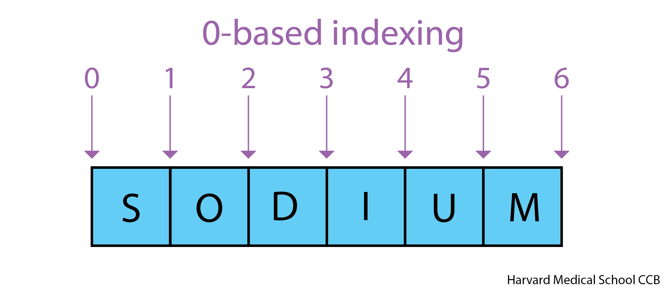
- The characters (individual letters, numbers, and so on) in a string
are ordered. For example, the string
'AB'is not the same as'BA'. Because of this ordering, we can treat the string as a list of characters. - Each position in the string (first, second, etc.) is given a number. This number is called an index or sometimes a subscript.
- Indices are numbered from 0.
- Use the position’s index in square brackets to get the character at that position.
OUTPUT
sUse a slice to get a substring.
- A part of a string is called a substring. A substring can be as short as a single character.
- An item in a list is called an element. Whenever we treat a string as if it were a list, the string’s elements are its individual characters.
- Slicing gets a part of a string (or, more generally, a part of any list-like thing).
- Slicing uses the notation
[start:stop], wherestartis the integer index of the first element we want andstopis the integer index of the element just after the last element we want. - The difference between
stopandstartis the slice’s length. - Taking a slice does not change the contents of the original string. Instead, taking a slice returns a copy of part of the original string.
OUTPUT
sodUse the built-in function len to find the length of a
string.
OUTPUT
6- Nested functions are evaluated from the inside out, like in mathematics.
Indexing
If you assign a = 123, what happens if you try to get
the second digit of a via a[1]?
Numbers are not strings or sequences and Python will raise an error
if you try to perform an index operation on a number. In the next
lesson on types and type conversion we will learn more about types
and how to convert between different types. If you want the Nth digit of
a number you can convert it into a string using the str
built-in function and then perform an index operation on that
string.
OUTPUT
TypeError: 'int' object is not subscriptableOUTPUT
2OUTPUT
atom_name[1:3] is: arSlicing concepts
Given the following string:
What would these expressions return?
species_name[2:8]-
species_name[11:](without a value after the colon) -
species_name[:4](without a value before the colon) -
species_name[:](just a colon) species_name[11:-3]species_name[-5:-3]- What happens when you choose a
stopvalue which is out of range? (i.e., tryspecies_name[0:20]orspecies_name[:103])
-
species_name[2:8]returns the substring'acia b' -
species_name[11:]returns the substring'folia', from position 11 until the end -
species_name[:4]returns the substring'Acac', from the start up to but not including position 4 -
species_name[:]returns the entire string'Acacia buxifolia' -
species_name[11:-3]returns the substring'fo', from the 11th position to the third last position -
species_name[-5:-3]also returns the substring'fo', from the fifth last position to the third last - If a part of the slice is out of range, the operation does not fail.
species_name[0:20]gives the same result asspecies_name[0:], andspecies_name[:103]gives the same result asspecies_name[:]
Content from Built-in Functions and Help
Last updated on 2023-04-14 | Edit this page
Overview
Questions
- How can I use built-in functions?
- How can I find out what they do?
- What kind of errors can occur in programs?
Objectives
- Explain the purpose of functions.
- Correctly call built-in Python functions.
- Correctly nest calls to built-in functions.
- Use help to display documentation for built-in functions.
- Correctly describe situations in which SyntaxError and NameError occur.
Key Points
- Use comments to add documentation to programs.
- A function may take zero or more arguments.
- Commonly-used built-in functions include
max,min, andround. - Functions may only work for certain (combinations of) arguments.
- Functions may have default values for some arguments.
- Use the built-in function
helpto get help for a function. - Python reports a syntax error when it can’t understand the source of a program.
- Python reports a runtime error when something goes wrong while a program is executing.
Use comments to add documentation to programs.
PYTHON
# This sentence isn't executed by Python.
adjustment = 0.5   # Neither is this - anything after '#' is ignored.
Comments are important for the readability of your code. They are where you can explain what your code is doing, decisions you made, and things to watch out for when using the code.
Well-commented code will be easier to use by others, and by you if you are returning to code you wrote months or years ago.
A function may take zero or more arguments.
- We have seen some functions already — now let’s take a closer look.
- An argument is a value passed into a function.
-
lentakes exactly one. -
int,str, andfloatcreate a new value from an existing one. -
printtakes zero or more. -
printwith no arguments prints a blank line.- Must always use parentheses, even if they’re empty, so that Python knows a function is being called.
OUTPUT
before

after
Every function returns something.
- Every function call produces some result.
- If the function doesn’t have a useful result to return, it usually
returns the special value
None.Noneis a Python object that stands in anytime there is no value.
Note that even though we set the result of print equal to a variable, printing still occurs.
OUTPUT
example
result of print is None
Commonly-used built-in functions include max,
min, and round.
- Use
maxto find the largest value of one or more values. - Use
minto find the smallest. - Both work on character strings as well as numbers.
- “Larger” and “smaller” use (0-9, A-Z, a-z) to compare letters.
OUTPUT
3
0
Functions may only work for certain (combinations of) arguments.
-
maxandminmust be given at least one argument.- “Largest of the empty set” is a meaningless question.
- And they must be given things that can meaningfully be compared.
ERROR
TypeError                                 Traceback (most recent call last)
<ipython-input-52-3f049acf3762> in <module>
----> 1 print(max(1, 'a'))

TypeError: '>' not supported between instances of 'str' and 'int'
Functions may have default values for some arguments.
-
roundwill round off a floating-point number. - By default, rounds to zero decimal places.
OUTPUT
4- We can specify the number of decimal places we want.
OUTPUT
3.7Functions attached to objects are called methods
- Functions take another form that will be common in the pandas episodes.
- Methods have parentheses like functions, but come after the variable.
- Some methods are used for internal Python operations, and are marked with double underlines.
PYTHON
my_string = 'Hello world!'  # creation of a string object

print(len(my_string))       # the len function takes a string as an argument and returns the length of the string

print(my_string.swapcase()) # calling the swapcase method on the my_string object

print(my_string.__len__())  # calling the internal __len__ method on the my_string object, used by len(my_string)
OUTPUT
12
hELLO WORLD!
12- You might even see them chained together. They operate left to right.
PYTHON
print(my_string.isupper())          # Not all the letters are uppercase
print(my_string.upper())            # This capitalizes all the letters

print(my_string.upper().isupper())  # Now all the letters are uppercase
OUTPUT
False
HELLO WORLD
True
Use the built-in function help to get help for a
function.
- Every built-in function has online documentation.
OUTPUT
Help on built-in function round in module builtins:

round(number, ndigits=None)
    Round a number to a given precision in decimal digits.

    The return value is an integer if ndigits is omitted or None.  Otherwise
    the return value has the same type as the number.  ndigits may be negative.
The Jupyter Notebook has two ways to get help.
- Option 1: Place the cursor near where the function is invoked in a
cell (i.e., the function name or its parameters),
- Hold down Shift, and press Tab.
- Do this several times to expand the information returned.
- Option 2: Type the function name in a cell with a question mark after it. Then run the cell.
Python reports a syntax error when it can’t understand the source of a program.
- Won’t even try to run the program if it can’t be parsed.
ERROR
  File "<ipython-input-56-f42768451d55>", line 2
    name = 'Feng
                ^
SyntaxError: EOL while scanning string literalERROR
  File "<ipython-input-57-ccc3df3cf902>", line 2
    age = = 52
          ^
SyntaxError: invalid syntax- Look more closely at the error message:
ERROR
  File "<ipython-input-6-d1cc229bf815>", line 1
    print ("hello world"
                        ^
SyntaxError: unexpected EOF while parsing- The message indicates a problem on first line of the input (“line
1”).
- In this case the “ipython-input” section of the file name tells us that we are working with input into IPython, the Python interpreter used by the Jupyter Notebook.
- The
-6-part of the filename indicates that the error occurred in cell 6 of our Notebook. - Next is the problematic line of code, indicating the problem with a
^pointer.
Python reports a runtime error when something goes wrong while a program is executing.
ERROR
NameError                                 Traceback (most recent call last)
<ipython-input-59-1214fb6c55fc> in <module>
      1 age = 53
----> 2 remaining = 100 - aege # mis-spelled 'age'

NameError: name 'aege' is not defined- Fix syntax errors by reading the source and runtime errors by tracing execution.
What Happens When
- Order of operations:
1.1 * radiance = 1.11.1 - 0.5 = 0.6min(radiance, 0.6) = 0.62.0 + 0.6 = 2.6max(2.1, 2.6) = 2.6
- At the end,
radiance = 2.6
Spot the Difference
- Predict what each of the
printstatements in the program below will print. - Does
max(len(rich), poor)run or produce an error message? If it runs, does its result make any sense?
OUTPUT
cmax for strings ranks them alphabetically.
OUTPUT
tinOUTPUT
4max(len(rich), poor) throws a TypeError. This turns into
max(4, 'tin') and as we discussed earlier a string and
integer cannot meaningfully be compared.
ERROR
TypeError                                 Traceback (most recent call last)
<ipython-input-65-bc82ad05177a> in <module>
----> 1 max(len(rich), poor)

TypeError: '>' not supported between instances of 'str' and 'int'
Why Not?
Why is it that max and min do not return
None when they are called with no arguments?
max and min return TypeErrors in this case
because the correct number of parameters was not supplied. If it just
returned None, the error would be much harder to trace as
it would likely be stored into a variable and used later in the program,
only to likely throw a runtime error.
Last Character of a String
If Python starts counting from zero, and len returns the
number of characters in a string, what index expression will get the
last character in the string name? (Note: we will see a
simpler way to do this in a later episode.)
Explore the Python docs!
The official Python documentation is arguably the most complete source of information about the language. It is available in different languages and contains a lot of useful resources. The Built-in Functions page contains a catalogue of all of these functions, including the ones that we’ve covered in this lesson. Some of these are more advanced and unnecessary at the moment, but others are very simple and useful.
Content from String Manipulation
Last updated on 2023-04-27 | Edit this page
Overview
Questions
- How can I manipulate text?
- How can I create neat and dynamic text output?
Objectives
- Extract substrings of interest.
- Format dynamic strings using f-strings.
- Explore Python’s built-in string functions
Key Points
- Strings can be indexed and sliced.
- Strings cannot be directly altered.
- You can build complex strings based on other variables using f-strings and format.
- Python has a variety of useful built-in string functions.
Strings can be indexed and sliced.
As we saw in class during the types lesson, strings in Python can be indexed and sliced
OUTPUT
'a'OUTPUT
'ha'OUTPUT
'Wha'OUTPUT
'hat a lovely day.'Strings are immutable.
We will talk about this concept in more detail when we explore lists. However, for now it is important to note that strings, like simple types, cannot have their values be altered in Python. Instead, a new value is created.
For simple types, this behavior isn’t that noticable:
PYTHON
x = 10
# While this line appears to be changing the value 10 to 11, in reality a new integer with the value 11 is created and assigned to x.
x = x + 1
x
OUTPUT
11However, for strings we can easily cause errors if we attempt to change them directly:
ERROR
---------------------------------------------------------------------
TypeError                           Traceback (most recent call last)
Input In [6], in <cell line: 1>()
----> 1 my_string[-1] = "g"

TypeError: 'str' object does not support item assignment
Thus, we need to learn ways in Python to manipulate and build strings. In this instance, we can build a new string using indexing:
OUTPUT
'What a lovely dag'Or use the built-in function str.replace() if we wanted
to replace a larger portion of the string.
OUTPUT
What a lovely dog.Build complex strings based on other variables using format.
What if we want to use values inside of a string? For instance, say we want to print a sentence denoting how many and the percent of samples we dropped and kept as a part of a quality control analysis.
Suppose we have variables denoting how many samples and dropped samples we have:
PYTHON
good_samples = 964
bad_samples = 117
percent_dropped = bad_samples/(good_samples + bad_samples)
One option would be to simply put everything in
print:
OUTPUT
Dropped 0.10823311748381129 percent samplesOr we could convert and use addition:
OUTPUT
Dropped 0.10823311748381129% samplesHowever, both of these options don’t give us as much control over how the percent is displayed. Python uses systems called string formatting and f-strings to give us greater control.
We can use Python’s built-in format function to create
better-looking text:
PYTHON
print('Dropped {0:.2%} of samples, with {1:n} samples remaining.'.format(percent_dropped, good_samples))OUTPUT
Dropped 10.82% of samples, with 964 samples remaining.Calls to format have a number of components:
- The use of brackets
{}to create replacement fields. - The index inside each bracket (0 and 1) to denote the index of the variable to use.
- Format instructions.
.2%indicates that we want to format the number as a percent with 2 decimal places.nindicates that we want to format as a number. -
formatwe call format on the string, and as arguments give it the variables we want to use. The order of variables here are the indices referenced in replacement fields.
For instance, we can switch or repeat indices:
PYTHON
print('Dropped {1:.2%} of samples, with {0:n} samples remaining.'.format(percent_dropped, good_samples))
print('Dropped {0:.2%} of samples, with {0:n} samples remaining.'.format(percent_dropped, good_samples))
OUTPUT
Dropped 96400.00% of samples, with 964 samples remaining.
Dropped 10.82% of samples, with 0.108233 samples remaining.
Python has a shorthand for using format called
f-strings. These strings let us directly use variables and
create expressions inside of strings. We denote an f-string
by putting f in front of the string definition:
PYTHON
print(f'Dropped {percent_dropped:.2%} of samples, with {good_samples:n} samples remaining.')
print(f'Dropped {100*(bad_samples/(good_samples + bad_samples)):.2f}% of samples, with {good_samples:n} samples remaining.')
OUTPUT
Dropped 10.82% of samples, with 964 samples remaining.
Dropped 10.82% of samples, with 964 samples remaining.
Here,
{100*(bad_samples/(good_samples + bad_samples)):.2f} is
treated as an expression, and then printed as a float
with 2 digits.
Full documenation on all of the string formatting mini-language can be found here.
Python has many useful built-in functions for string manipulation.
Python has many built-in methods for manipulating strings; simple and powerful text manipulation is considered one of Python’s strengths. We will go over some of the more common and useful functions here, but be aware that there are many more you can find in the official documentation.
Dealing with whitespace
str.strip() strips the whitespace from the beginning and
ending of a string. This is especially useful when reading in files
which might have hidden spaces or tabs at the end of lines.
Note that \t denotes a tab character.
OUTPUT
'a'str.split() strips a string up into a list of strings by
some character. By default it uses whitespace, but we can give any set
character to split by. We will learn how to use lists in the next
session.
OUTPUT
['My',
 'favorite',
 'sentence',
 'I',
 'hope',
 'nothing',
 'bad',
 'happens',
 'to',
'it']OUTPUT
['2023', '04', '12']Pattern matching
str.find() find the first occurrence of the specified
string inside the search string, and str.rfind() finds the
last.
OUTPUT
11OUTPUT
38str.startswith() and str.endswith() perform
a simlar function but return a bool based on whether or not
the string starts or ends with a particular string.
OUTPUT
FalseOUTPUT
TrueCase
str.upper(), str.lower(),
str.capitalize(), and str.title() all change
the capitalization of strings.
PYTHON
my_string = "liters (coffee) per minute"
print(my_string.lower())
print(my_string.upper())
print(my_string.capitalize())
print(my_string.title())
OUTPUT
liters (coffee) per minute
LITERS (COFFEE) PER MINUTE
Liters (coffee) per minute
Liters (Coffee) Per Minute
Challenge
A common problem when analyzing data is that multiple features of the data will be stored as a column name or single string.
For instance, consider the following column headers:
WT_0Min_1 WT_0Min_2 X.RAB7A_0Min_1 X.RAB7A_0Min_2 WT_5Min_1 WT_5Min_2 X.RAB7A_5Min_1 X.RAB7A_5Min_2 X.NPC1_5Min_1 X.NPC1_5Min_2There are two variables of interest, the time, 0, 5, or 60 minutes post-infection, and the genotype, WT, NPC1 knockout and RAB7A knockout. We also have replicate information at the end of each column header. For now, let’s just try extracting the timepoint, genotype, and replicate from a single column header.
Given the string:
Try to print the string:
Sample is 0min RABA7A knockout, replicate 1. Using f-strings, slicing and indexing, and built-in string functions.
You can try to use lists as a challenge, but its fine to instead get
each piece of information separately from sample_info.
Content from Using Objects
Last updated on 2023-04-20 | Edit this page
Overview
Questions
- What is an object?
Objectives
- Define objects.
- Use an object’s methods.
- Call a constructor for an object.
Key Points
- Objects are entities with both data and methods
- Methods are unique to objects, and so methods with the same name may work differently on different objects.
- You can create an object using a constructor.
- Objects need to be explicitly copied.
Objects are entities with both data and methods
In addition to basic types, Python also has objects we refer to the type of an object as its class. In other programming languages there is a more definite distinction between base types and objects, but in Python these terms essentially interchangable. However, thinking about more complex data structures through an object-oriented lense will allow us to better understand how to write effective code.
We can think of an object as an entity which has two aspects: data and methods. The data (sometimes called properties) is what we would typically think of as the value of that object; what it is storing. Methods define what we can do with an object, essentially they are functions specific to an object (you will often hear function and method used interchangebly).
Next session we will explore the list object in Python.
A list consists of its data, or what is stored in the list.
PYTHON
# Here, we are storing 3, 67, 1, and 33 as the data inside the list object
sizes = [3,67,1,33]

# Reverse is a list method which reverses that list
sizes.reverse()

print(sizes)
OUTPUT
[33, 1, 67, 3]Methods are unique to objects, and so methods with the same name may work differently on different objects.
In Python, many objects share method names. However, those methods may do different things.
We have already seen this implicitly looking at how operations like addition interact with different basic types. For instance, performing multiplication on a list:
OUTPUT
[33, 1, 67, 3, 33, 1, 67, 3, 33, 1, 67, 3]May not have the behavior you expect. Whenever our code isn’t doing
what we want, one of the first things to check is that the
type of our variables is what we expect.
You can create an object using a constructor.
All objects have constructors, which are special function that create
that object. Constructors are often called implicitly when we, for
instance, define a list using the [] notation or create a
Pandas dataframe object using read_csv.
However, objects also have explicit constructors which can be called
directly.
PYTHON
# The basic list constructor
new_sizes = list()

new_sizes.append(33)
new_sizes.append(1)
new_sizes.append(67)
new_sizes.append(3)

print(new_sizes)
OUTPUT
[33, 1, 67, 3]Objects need to be explicitly copied.
We will continue to circle back to this point, but one imporant note about complex objects is that they need to be explicitly copied. This is due to them being mutable, which we will discuss more next session.
We can have multiple variables refer to the same object. This can result in us unknowningly changing an object we didn’t expect to.
For instance, two variables can refer to the same list:
PYTHON
# Here, we lose the original sizes list and now both variables are pointing to the same list
sizes = new_sizes
print(sizes)
print(new_sizes)

# Thus, if we change sizes:
sizes.append(100)

# We see that new_sizes has also changed
print(sizes)
print(new_sizes)
OUTPUT
[33, 1, 67, 3]
[33, 1, 67, 3]
[33, 1, 67, 3, 100]
[33, 1, 67, 3, 100]
In order to make a variable refer to a different copy of a list, we need to explicitly copy it. One way to do this is to use a copy constructor. Most objects in Python have a copy constructor which accepts another object of the same type and creates a copy of it.
PYTHON
# Calling the copy constructor
sizes = list(new_sizes)
print(sizes)
print(new_sizes)

# Now if we change sizes:
sizes.append(100)

# We see that new_sizes does NOT change
print(sizes)
print(new_sizes)
OUTPUT
[33, 1, 67, 3, 100]
[33, 1, 67, 3, 100]
[33, 1, 67, 3, 100, 100]
[33, 1, 67, 3, 100]
However, even copying an object can sometimes not be enough. Some objects are able to store other objects. If this is the case, the internal object might not change.
OUTPUT
[[33, 1, 67, 3, 100, 100], [33, 1, 67, 3, 100, 100], [33, 1, 67, 3, 100, 100], [33, 1, 67, 3, 100, 100]]PYTHON
# While the external list here is different, the internal lists are still the same
new_lol = list(list_of_lists)
print(new_lol)
OUTPUT
[[33, 1, 67, 3, 100, 100], [33, 1, 67, 3, 100, 100], [33, 1, 67, 3, 100, 100], [33, 1, 67, 3, 100, 100]]OUTPUT
[[100, 3, 67, 1, 33], [100, 3, 67, 1, 33], [100, 3, 67, 1, 33], [100, 3, 67, 1, 33]]Overall, we need to be careful in Python when copying objects. This is one of the reasons why most libaries’ methods return new objects as opposed to altering existing objects, so as to avoid any confusion over different object versions. Additionally, we can perform a deep copy of an object, which is an object copy which copys and stored objects.
Challenge
Pandas is one of the most popular python libraries for manipulating data which we will be diving into next week. Take a look at the official documentation for Pandas and try to find how to create a deep copy of a dataframe. Is what you found a function or a method? You can find the documentation here
Dataframes in Pandas have a copy method found
here.
This method by default performs a deep copy as the deep
argument’s default value is True.
Content from Lists
Last updated on 2023-04-20 | Edit this page
Overview
Questions
- How can I store many values together?
- How do I access items stored in a list?
- How are variables assigned to lists different than variables assigned to values?
Objectives
- Explain what a list is.
- Create and index lists of simple values.
- Change the values of individual elements
- Append values to an existing list
- Reorder and slice list elements
- Create and manipulate nested lists
Key Points
-
[value1, value2, value3, ...]creates a list. - Lists can contain any Python object, including lists (i.e., list of lists).
- Lists are indexed and sliced with square brackets (e.g., list[0] and list[2:9]), in the same way as strings and arrays.
- Lists are mutable (i.e., their values can be changed in place).
- Strings are immutable (i.e., the characters in them cannot be changed).
Python lists
We create a list by putting values inside square brackets and separating the values with commas:
OUTPUT
odds are: [1, 3, 5, 7]The empty list
Similar to an empty string, we can create an empty list with a
len of 0 and no elements. We create an empty list as
empty_list = [] or empty_list = list(), and it
is useful when we want to build up a list element by element.
We can access elements of a list using indices – numbered positions of elements in the list. These positions are numbered starting at 0, so the first element has an index of 0.
PYTHON
print('first element:', odds[0])
print('last element:', odds[3])
print('"-1" element:', odds[-1])
OUTPUT
first element: 1
last element: 7
"-1" element: 7
Yes, we can use negative numbers as indices in Python. When we do so,
the index -1 gives us the last element in the list,
-2 the second to last, and so on. Because of this,
odds[3] and odds[-1] point to the same element
here.
There is one important difference between lists and strings: we can change the values in a list, but we cannot change individual characters in a string. For example:
PYTHON
names = ['Curie', 'Darwing', 'Turing']  # typo in Darwin's name
print('names is originally:', names)
names[1] = 'Darwin'  # correct the name
print('final value of names:', names)
OUTPUT
names is originally: ['Curie', 'Darwing', 'Turing']
final value of names: ['Curie', 'Darwin', 'Turing']
works, but:
ERROR
---------------------------------------------------------------------------
TypeError                                 Traceback (most recent call last)
<ipython-input-8-220df48aeb2e> in <module>()
     1 name = 'Darwin'
----> 2 name[0] = 'd'

TypeError: 'str' object does not support item assignment
does not. This is because a list is mutable while a string is immutable.
Mutable and immutable
Data which can be modified in place is called mutable, while data which cannot be modified is called immutable. Strings and numbers are immutable. This does not mean that variables with string or number values are constants, but when we want to change the value of a string or number variable, we can only replace the old value with a completely new value.
Lists and arrays, on the other hand, are mutable: we can modify them after they have been created. We can change individual elements, append new elements, or reorder the whole list. For some operations, like sorting, we can choose whether to use a function that modifies the data in-place or a function that returns a modified copy and leaves the original unchanged.
Be careful when modifying data in-place. If two variables refer to the same list, and you modify the list value, it will change for both variables!
PYTHON
mild_salsa = ['peppers', 'onions', 'cilantro', 'tomatoes']
hot_salsa = mild_salsa        # <-- mild_salsa and hot_salsa point to the *same* list data in memory
hot_salsa[0] = 'hot peppers'
print('Ingredients in mild salsa:', mild_salsa)
print('Ingredients in hot salsa:', hot_salsa)
OUTPUT
Ingredients in mild salsa: ['hot peppers', 'onions', 'cilantro', 'tomatoes']
Ingredients in hot salsa: ['hot peppers', 'onions', 'cilantro', 'tomatoes']
Let’s go to this link to visualize this code.
If you want variables with mutable values to be independent, you must make a copy of the value when you assign it.
PYTHON
mild_salsa = ['peppers', 'onions', 'cilantro', 'tomatoes']
hot_salsa = list(mild_salsa)        # <-- makes a *copy* of the list
hot_salsa[0] = 'hot peppers'
print('Ingredients in mild salsa:', mild_salsa)
print('Ingredients in hot salsa:', hot_salsa)
OUTPUT
Ingredients in mild salsa: ['peppers', 'onions', 'cilantro', 'tomatoes']
Ingredients in hot salsa: ['hot peppers', 'onions', 'cilantro', 'tomatoes']
Because of pitfalls like this, code which modifies data in place can be more difficult to understand. However, it is often far more efficient to modify a large data structure in place than to create a modified copy for every small change. You should consider both of these aspects when writing your code.
Nested Lists
Since a list can contain any Python variables, it can even contain other lists.
For example, you could represent the products on the shelves of a
small grocery shop as a nested list called veg:
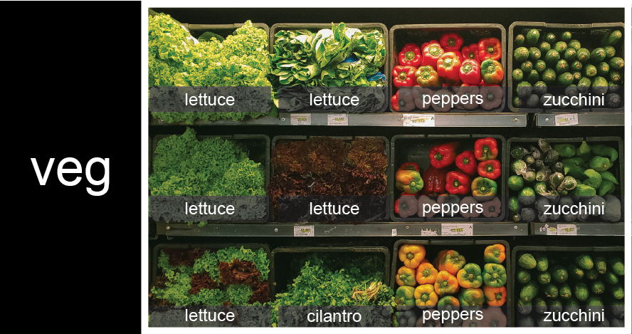
veg is represented as a shelf full
of produce. There are three rows of vegetables on the shelf, and each
row contains three baskets of vegetables. We can label each basket
according to the type of vegetable it contains, so the top row contains
(from left to right) lettuce, lettuce, and peppers.To store the contents of the shelf in a nested list, you write it this way:
PYTHON
veg = [['lettuce', 'lettuce', 'peppers', 'zucchini'],
    ['lettuce', 'lettuce', 'peppers', 'zucchini'],
    ['lettuce', 'cilantro', 'peppers', 'zucchini']]
Here are some visual examples of how indexing a list of lists
veg works. First, you can reference each row on the shelf
as a separate list. For example, veg[2] represents the
bottom row, which is a list of the baskets in that row.
![veg is now shown as a list of three rows, with veg[0] representing the top row of three baskets, veg[1] representing the second row, and veg[2] representing the bottom row.](fig/05_groceries_veg0.png)
veg is now shown as a list of three
rows, with veg[0] representing the top row of three
baskets, veg[1] representing the second row, and
veg[2] representing the bottom row.Index operations using the image would work like this:
OUTPUT
['lettuce', 'cilantro', 'peppers', 'zucchini']OUTPUT
['lettuce', 'lettuce', 'peppers', 'zucchini']To reference a specific basket on a specific shelf, you use two
indexes. The first index represents the row (from top to bottom) and the
second index represents the specific basket (from left to right). ![veg is now shown as a two-dimensional grid, with each basket labeled according to its index in the nested list. The first index is the row number and the second index is the basket number, so veg[1][3] represents the basket on the far right side of the second row (basket 4 on row 2): zucchini](fig/05_groceries_veg00.png)
OUTPUT
'lettuce'OUTPUT
'peppers'Manipulating Lists
There are many ways to change the contents of lists besides assigning new values to individual elements:
OUTPUT
odds after adding a value: [1, 3, 5, 7, 11]PYTHON
removed_element = odds.pop(0)
print('odds after removing the first element:', odds)
print('removed_element:', removed_element)
OUTPUT
odds after removing the first element: [3, 5, 7, 11]
removed_element: 1OUTPUT
odds after reversing: [11, 7, 5, 3]While modifying in place, it is useful to remember that Python treats lists in a slightly counter-intuitive way.
As we saw earlier, when we modified the mild_salsa list
item in-place, if we make a list, (attempt to) copy it and then modify
this list, we can cause all sorts of trouble. This also applies to
modifying the list using the above functions:
PYTHON
odds = [3, 5, 7]
primes = odds
primes.append(2)
print('primes:', primes)
print('odds:', odds)
OUTPUT
primes: [3, 5, 7, 2]
odds: [3, 5, 7, 2]
This is because Python stores a list in memory, and then can use
multiple names to refer to the same list. If all we want to do is copy a
(simple) list, we can again use the list function, so we do
not modify a list we did not mean to:
PYTHON
odds = [3, 5, 7]
primes = list(odds)
primes.append(2)
print('primes:', primes)
print('odds:', odds)
OUTPUT
primes: [3, 5, 7, 2]
odds: [3, 5, 7]
Subsets of lists can be accessed by slicing, similar to how we accessed ranges of positions in a strings.
PYTHON
binomial_name = 'Drosophila melanogaster'
genus = binomial_name[0:10]
print('genus:', genus)

species = binomial_name[11:23]
print('species:', species)

chromosomes = ['X', 'Y', '2', '3', '4']
autosomes = chromosomes[2:5]
print('autosomes:', autosomes)

last = chromosomes[-1]
print('last:', last)
OUTPUT
genus: Drosophila
species: melanogaster
autosomes: ['2', '3', '4']
last: 4
Slicing From the End
Use slicing to access only the last four characters of a string or entries of a list.
PYTHON
string_for_slicing = 'Observation date: 02-Feb-2013'
list_for_slicing = [['fluorine', 'F'],
                   ['chlorine', 'Cl'],
                   ['bromine', 'Br'],
                   ['iodine', 'I'],
                   ['astatine', 'At']]
Desired output:
OUTPUT
'2013'
[['chlorine', 'Cl'], ['bromine', 'Br'], ['iodine', 'I'], ['astatine', 'At']]
Would your solution work regardless of whether you knew beforehand the length of the string or list (e.g. if you wanted to apply the solution to a set of lists of different lengths)? If not, try to change your approach to make it more robust.
Hint: Remember that indices can be negative as well as positive
Non-Continuous Slices
So far we’ve seen how to use slicing to take single blocks of successive entries from a sequence. But what if we want to take a subset of entries that aren’t next to each other in the sequence?
You can achieve this by providing a third argument to the range within the brackets, called the step size. The example below shows how you can take every third entry in a list:
PYTHON
primes = [2, 3, 5, 7, 11, 13, 17, 19, 23, 29, 31, 37]
subset = primes[0:12:3]
print('subset', subset)
OUTPUT
subset [2, 7, 17, 29]Notice that the slice taken begins with the first entry in the range, followed by entries taken at equally-spaced intervals (the steps) thereafter. If you wanted to begin the subset with the third entry, you would need to specify that as the starting point of the sliced range:
PYTHON
primes = [2, 3, 5, 7, 11, 13, 17, 19, 23, 29, 31, 37]
subset = primes[2:12:3]
print('subset', subset)
OUTPUT
subset [5, 13, 23, 37]Use the step size argument to create a new string that contains only every other character in the string “In an octopus’s garden in the shade”. Start with creating a variable to hold the string:
What slice of beatles will produce the following output
(i.e., the first character, third character, and every other character
through the end of the string)?
OUTPUT
I notpssgre ntesaeIf you want to take a slice from the beginning of a sequence, you can omit the first index in the range:
PYTHON
date = 'Monday 4 January 2016'
day = date[0:6]
print('Using 0 to begin range:', day)
day = date[:6]
print('Or omit the beginning index to slice from 0:', day)
OUTPUT
Using 0 to begin range: Monday
Or omit the beginning index to slice from 0: Monday
And similarly, you can omit the ending index in the range to take a slice to the very end of the sequence:
PYTHON
months = ['jan', 'feb', 'mar', 'apr', 'may', 'jun', 'jul', 'aug', 'sep', 'oct', 'nov', 'dec']
sond = months[8:12]
print('With known last position:', sond)
sond = months[8:len(months)]
print('Using len() to get last entry:', sond)
sond = months[8:]
print('Or omit the final index to go to the end of the list:', sond)
OUTPUT
With known last position: ['sep', 'oct', 'nov', 'dec']
Using len() to get last entry: ['sep', 'oct', 'nov', 'dec']
Or omit the final index to go to the end of the list: ['sep', 'oct', 'nov', 'dec']
Going past len
Python does not consider it an error to go past the end of a list when slicing. Python will juse slice until the end of the list:
OUTPUT
['jan', 'feb', 'mar', 'apr', 'may', 'jun', 'jul', 'aug', 'sep', 'oct', 'nov', 'dec']However, trying to get a single item from a list at an index greater than its length will result in an error:
ERROR
---------------------------------------------------------------------------
IndexError                                Traceback (most recent call last)
Input In [5], in <cell line: 1>()
----> 1 months[30]

IndexError: list index out of range
Overloading
+ usually means addition, but when used on strings or
lists, it means “concatenate”. Given that, what do you think the
multiplication operator * does on lists? In particular,
what will be the output of the following code?
[2, 4, 6, 8, 10, 2, 4, 6, 8, 10][4, 8, 12, 16, 20][[2, 4, 6, 8, 10],[2, 4, 6, 8, 10]][2, 4, 6, 8, 10, 4, 8, 12, 16, 20]
The technical term for this is operator overloading: a
single operator, like + or *, can do different
things depending on what it’s applied to.
Content from For Loops
Last updated on 2023-04-20 | Edit this page
Overview
Questions
- How can I make a program do many things?
- How can I do something for each thing in a list?
Objectives
- Explain what for loops are normally used for.
- Trace the execution of a simple (unnested) loop and correctly state the values of variables in each iteration.
- Write for loops that use the Accumulator pattern to aggregate values.
Key Points
- A for loop executes commands once for each value in a collection.
- A
forloop is made up of a collection, a loop variable, and a body. - The first line of the
forloop must end with a colon, and the body must be indented. - Indentation is always meaningful in Python.
- Loop variables can be called anything (but it is strongly advised to have a meaningful name to the looping variable).
- The body of a loop can contain many statements.
- Use
rangeto iterate over a sequence of numbers.
A for loop executes commands once for each value in a collection.
- Doing calculations on the values in a list one by one is as painful
as working with
pressure_001,pressure_002, etc. - A for loop tells Python to execute some statements once for each value in a list, a character string, or some other collection.
- “for each thing in this group, do these operations”
- This
forloop is equivalent to:
- And the
forloop’s output is:
OUTPUT
2
3
5
A for loop is made up of a collection, a loop variable,
and a body.
- The collection,
[2, 3, 5], is what the loop is being run on. - The body,
print(number), specifies what to do for each value in the collection. - The loop variable,
number, is what changes for each iteration of the loop.- The “current thing”.
The first line of the for loop must end with a colon,
and the body must be indented.
- The colon at the end of the first line signals the start of a block of statements.
- Python uses indentation rather than
{}orbegin/endto show nesting.- Any consistent indentation is legal, but almost everyone uses four spaces.
OUTPUT
IndentationError: expected an indented block- Indentation is always meaningful in Python.
ERROR
  File "<ipython-input-7-f65f2962bf9c>", line 2
    lastName = "Smith"
    ^
IndentationError: unexpected indent- This error can be fixed by removing the extra spaces at the beginning of the second line.
Loop variables can be called anything.
- As with all variables, loop variables are:
- Created on demand.
- Meaningless: their names can be anything at all.
The body of a loop can contain many statements.
- But no loop should be more than a few lines long.
- Hard for human beings to keep larger chunks of code in mind.
OUTPUT
2 4 8
3 9 27
5 25 125
Use range to iterate over a sequence of numbers.
- The built-in function
rangeproduces a sequence of numbers.- Not a list: the numbers are produced on demand to make looping over large ranges more efficient.
-
range(N)is the numbers 0..N-1- Exactly the legal indices of a list or character string of length N
OUTPUT
a range is not a list: range(0, 3)
0
1
2
The Accumulator pattern turns many values into one.
- A common pattern in programs is to:
- Initialize an accumulator variable to zero, the empty string, or the empty list.
- Update the variable with values from a collection.
PYTHON
# Sum the first 5 integers.
my_sum = 0 # Line 1
for number in range(5): # Line 2
   my_sum = my_sum + (number + 1) # Line 3
print(my_sum) # Line 4
OUTPUT
15- Read
total = total + (number + 1)as:- Add 1 to the current value of the loop variable
number. - Add that to the current value of the accumulator variable
total. - Assign that to
total, replacing the current value.
- Add 1 to the current value of the loop variable
- We have to add
number + 1becauserangeproduces 0..9, not 1..10.- You could also have used
numberandrange(11).
- You could also have used
We can trace the program output by looking at which line of code is being executed and what each variable’s value is at each line:
| Line No | Variables |
|---|---|
| 1 | my_sum = 0 |
| 2 | my_sum = 0 number = 0 |
| 3 | my_sum = 1 number = 0 |
| 2 | my_sum = 1 number = 1 |
| 3 | my_sum = 3 number = 1 |
| 2 | my_sum = 3 number = 2 |
| 3 | my_sum = 6 number = 2 |
| 2 | my_sum = 6 number = 3 |
| 3 | my_sum = 10 number = 3 |
| 2 | my_sum = 10 number = 4 |
| 3 | my_sum = 15 number = 4 |
| 4 | my_sum = 15 number = 4 |
Let’s double check our work by visualizing the code.
Classifying Errors
Is an indentation error a syntax error or a runtime error?
An indentation error (IndentationError) is a syntax
error. Programs with syntax errors cannot be started. A program with a
runtime error will start but an error will be thrown under certain
conditions.
| Line no | Variables |
|---|---|
| 1 | total = 0 |
| 2 | total = 0 char = ‘t’ |
| 3 | total = 1 char = ‘t’ |
| 2 | total = 1 char = ‘i’ |
| 3 | total = 2 char = ‘i’ |
| 2 | total = 2 char = ‘n’ |
| 3 | total = 3 char = ‘n’ |
Practice Accumulating
Fill in the blanks in each of the programs below to produce the indicated result.
PYTHON
# A
# Total length of the strings in the list: ["red", "green", "blue"] => 12
total = 0
for word in ["red", "green", "blue"]:
    ____ = ____ + len(word)
print(total)

# B
# Concatenate all words: ["red", "green", "blue"] => "redgreenblue"
words = ["red", "green", "blue"]
result = ____
for ____ in ____:
    ____
print(result)

# C
# List of word lengths: ["red", "green", "blue"] => [3, 5, 4]
lengths = ____
for word in ["red", "green", "blue"]:
    lengths.____(____)
print(lengths)PYTHON
# A
# Total length of the strings in the list: ["red", "green", "blue"] => 12
total = 0
for word in ["red", "green", "blue"]:
    total = total + len(word)
print(total)

# B
# Concatenate all words: ["red", "green", "blue"] => "redgreenblue"
words = ["red", "green", "blue"]
result = ""
for word in words:
    result = result + word
print(result)

# C
# List of word lengths: ["red", "green", "blue"] => [3, 5, 4]
lengths = []
for word in ["red", "green", "blue"]:
    lengths.append(len(word))
print(lengths)
String accumulation
Starting from the list ["red", "green", "blue"], create
the acronym "RGB" using a for loop.
You may need to use a string method to properly format the acronym.
Identifying Variable Name Errors
- Read the code below and try to identify what the errors are without running it.
- Run the code and read the error message. What type of
NameErrordo you think this is? Is it a string with no quotes, a misspelled variable, or a variable that should have been defined but was not? - Fix the error.
- Repeat steps 2 and 3, until you have fixed all the errors.
This is a first taste of if statements. We will be going into more detail on if statements in future lessons. No errors in this code have to do with how the if statement is being used.
- Python variable names are case sensitive:
numberandNumberrefer to different variables. - The variable
messageneeds to be initialized as an empty string. - We want to add the string
"a"tomessage, not the undefined variablea.
Content from Libraries
Last updated on 2023-04-20 | Edit this page
Overview
Questions
- How can I use software that other people have written?
- How can I find out what that software does?
Objectives
- Explain what software libraries are and why programmers create and use them.
- Write programs that import and use modules from Python’s standard library.
- Find and read documentation for the standard library interactively (in the interpreter) and online.
Key Points
- Most of the power of a programming language is in its libraries.
- A program must import a library module in order to use it.
- Use
helpto learn about the contents of a library module. - Import specific items from a library to shorten programs.
- Create an alias for a library when importing it to shorten programs.
Most of the power of a programming language is in its libraries.
- A library is a collection of files (called
modules) that contains functions for use by other programs.
- May also contain data values (e.g., numerical constants) and other things.
- Library’s contents are supposed to be related, but there’s no way to enforce that.
- The Python standard library is an extensive suite of modules that comes with Python itself.
- Many additional libraries are available from PyPI (the Python Package Index).
Libraries, packages, and modules
A module is a typically defined set of code located within a single Python file which is intended to be imported into scripts or other modules. A package is a set of related modules, often contained in a single directory. A library is a more general term referring to a collection of modules and packages. For instance, the Python Standard Library contains functionality from compressing files to parallel programming.
However, these definitions are not particularly formal or strict. Module, package, and library are often used interchangeably, especially since many libraries only consist of a single module.
A program must import a library module before using it.
- Use
importto load a library module into a program’s memory. - Then refer to things from the module as
module_name.thing_name.- Python uses
.to mean “part of”.
- Python uses
- Using
math, one of the modules in the standard library:
OUTPUT
pi is 3.141592653589793
cos(pi) is -1.0- Have to refer to each item with the module’s name.
-
math.cos(pi)won’t work: the reference topidoesn’t somehow “inherit” the function’s reference tomath.
-
Use help to learn about the contents of a library
module.
- Works just like help for a function.
OUTPUT
Help on module math:

NAME
    math

MODULE REFERENCE
    http://docs.python.org/3/library/math

    The following documentation is automatically generated from the Python
    source files.  It may be incomplete, incorrect or include features that
    are considered implementation detail and may vary between Python
    implementations.  When in doubt, consult the module reference at the
    location listed above.

DESCRIPTION
    This module is always available.  It provides access to the
    mathematical functions defined by the C standard.

FUNCTIONS
    acos(x, /)
        Return the arc cosine (measured in radians) of x.
Import specific items from a library module to shorten programs.
- Use
from ... import ...to load only specific items from a library module. - Then refer to them directly without library name as prefix.
OUTPUT
cos(pi) is -1.0Create an alias for a library module when importing it to shorten programs.
- Use
import ... as ...to give a library a short alias while importing it. - Then refer to items in the library using that shortened name.
OUTPUT
cos(pi) is -1.0- Allows less typing for long and/or frequently used packages.
- E.g., the
matplotlib.pyplotplotting package is often aliased asplt.
- E.g., the
- But can make programs harder to understand, since readers must learn your program’s aliases.
Exploring the Math Module
- What function from the
mathmodule can you use to calculate a square root without usingsqrt? - Since the library contains this function, why does
sqrtexist?
Using
help(math)we see that we’ve gotpow(x,y)in addition tosqrt(x), so we could usepow(x, 0.5)to find a square root.-
The
sqrt(x)function is arguably more readable thanpow(x, 0.5)when implementing equations. Readability is a cornerstone of good programming, so it makes sense to provide a special function for this specific common case.Also, the design of Python’s
mathlibrary has its origin in the C standard, which includes bothsqrt(x)andpow(x,y), so a little bit of the history of programming is showing in Python’s function names.
Locating the Right Module
You want to select a random character from a string:
- Which standard library module could help you?
- Which function would you select from that module? Are there alternatives?
- Try to write a program that uses the function.
While you can use help from within Jupyter Lab, often
when working with Python searching on the internet can yield a faster
result.
The random module seems like it could help.
The string has 11 characters, each having a positional index from 0
to 10. You could use the random.randrange
or random.randint
functions to get a random integer between 0 and 10, and then select the
bases character at that index:
or more compactly:
Perhaps you found the random.sample
function? It allows for slightly less typing but might be a bit harder
to understand just by reading:
The simplest and shortest solution is the random.choice
function that does exactly what we want:
Jigsaw Puzzle (Parson’s Problem) Programming Example
Rearrange the following statements so that a random DNA base is printed and its index in the string. Not all statements may be needed. Feel free to use/add intermediate variables.
When Is Help Available?
When a colleague of yours types help(math), Python
reports an error:
OUTPUT
NameError: name 'math' is not definedWhat has your colleague forgotten to do?
Importing the math module (import math)
can be written as
Since you just wrote the code and are familiar with it, you might actually find the first version easier to read. But when trying to read a huge piece of code written by someone else, or when getting back to your own huge piece of code after several months, non-abbreviated names are often easier, except where there are clear abbreviation conventions.
There Are Many Ways To Import Libraries!
Match the following print statements with the appropriate library calls.
Print commands:
print("sin(pi/2) =", sin(pi/2))print("sin(pi/2) =", m.sin(m.pi/2))print("sin(pi/2) =", math.sin(math.pi/2))
Library calls:
from math import sin, piimport mathimport math as mfrom math import *
- Library calls 1 and 4. In order to directly refer to
sinandpiwithout the library name as prefix, you need to use thefrom ... import ...statement. Whereas library call 1 specifically imports the two functionssinandpi, library call 4 imports all functions in themathmodule. - Library call 3. Here
sinandpiare referred to with a shortened library nameminstead ofmath. Library call 3 does exactly that using theimport ... as ...syntax - it creates an alias formathin the form of the shortened namem. - Library call 2. Here
sinandpiare referred to with the regular library namemath, so the regularimport ...call suffices.
Note: although library call 4 works, importing all
names from a module using a wildcard import is not recommended as it makes it
unclear which names from the module are used in the code. In general it
is best to make your imports as specific as possible and to only import
what your code uses. In library call 1, the import
statement explicitly tells us that the sin function is
imported from the math module, but library call 4 does not
convey this information.
Most likely you find this version easier to read since it’s less
dense. The main reason not to use this form of import is to avoid name
clashes. For instance, you wouldn’t import degrees this way
if you also wanted to use the name degrees for a variable
or function of your own. Or if you were to also import a function named
degrees from another library.
OUTPUT
---------------------------------------------------------------------------
ValueError                                Traceback (most recent call last)
<ipython-input-1-d72e1d780bab> in <module>
      1 from math import log
----> 2 log(0)

ValueError: math domain error- The logarithm of
xis only defined forx > 0, so 0 is outside the domain of the function. - You get an error of type
ValueError, indicating that the function received an inappropriate argument value. The additional message “math domain error” makes it clearer what the problem is.
Content from Reading tabular data
Last updated on 2023-04-20 | Edit this page
Overview
Questions
- How can I read tabular data?
Objectives
- Import the Pandas library.
- Use Pandas to load a simple CSV data set.
- Get some basic information about a Pandas DataFrame.
Key Points
- Use the Pandas library to get basic statistics out of tabular data.
- Use
index_colto specify that a column’s values should be used as row headings. - Use
DataFrame.infoto find out more about a dataframe. - The
DataFrame.columnsvariable stores information about the dataframe’s columns. - Use
DataFrame.Tto transpose a dataframe. - Use
DataFrame.describeto get summary statistics about data.
Use the Pandas library to do statistics on tabular data.
- Pandas is a widely-used Python library for statistics, particularly on tabular data.
- Borrows many features from R’s dataframes.
- A 2-dimensional table whose columns have names and potentially have different data types.
- Load it with
import pandas as pd. The alias pd is commonly used for Pandas. - Read a Comma Separated Values (CSV) data file with
pd.read_csv.- Argument is the name of the file to be read.
- Assign result to a variable to store the data that was read.
Data description
We are going to use part of the data published by Blackmore et al. (2017), The effect of upper-respiratory infection on transcriptomic changes in the CNS. The goal of the study was to determine the effect of an upper-respiratory infection on changes in RNA transcription occurring in the cerebellum and spinal cord post infection. Gender matched eight week old C57BL/6 mice were inoculated with saline or with Influenza A by intranasal route and transcriptomic changes in the cerebellum and spinal cord tissues were evaluated by RNA-seq at days 0 (non-infected), 4 and 8.
The dataset is stored as a comma-separated values (CSV) file. Each row holds information for a single RNA expression measurement, and the first eleven columns represent:
| Column | Description |
|---|---|
| gene | The name of the gene that was measured |
| sample | The name of the sample the gene expression was measured in |
| expression | The value of the gene expression |
| organism | The organism/species - here all data stem from mice |
| age | The age of the mouse (all mice were 8 weeks here) |
| sex | The sex of the mouse |
| infection | The infection state of the mouse, i.e. infected with Influenza A or not infected. |
| strain | The Influenza A strain; C57BL/6 in all cases. |
| time | The duration of the infection (in days). |
| tissue | The tissue that was used for the gene expression experiment, i.e. cerebellum or spinal cord. |
| mouse | The mouse unique identifier. |
We will be seeing different parts of this total dataset in different lessons, such as just the expression data or sample data. Later, we will learn how to convert between these different data layouts. For this lesson, we will only be using a subset of the total dataset.
PYTHON
import pandas as pd

url = "https://raw.githubusercontent.com/ccb-hms/workbench-python-workshop/main/episodes/data/rnaseq_reduced.csv"
rnaseq_df = pd.read_csv(url)
print(rnaseq_df)
OUTPUT
         gene      sample  expression  time
0         Asl  GSM2545336        1170     8
1        Apod  GSM2545336       36194     8
2     Cyp2d22  GSM2545336        4060     8
3        Klk6  GSM2545336         287     8
4       Fcrls  GSM2545336          85     8
...       ...         ...         ...   ...
7365    Mgst3  GSM2545340        1563     4
7366   Lrrc52  GSM2545340           2     4
7367     Rxrg  GSM2545340          26     4
7368    Lmx1a  GSM2545340          81     4
7369     Pbx1  GSM2545340        3805     4

[7370 rows x 4 columns]
- The columns in a dataframe are the observed variables, and the rows are the observations.
- Pandas uses backslash
\to show wrapped lines when output is too wide to fit the screen.
Use index_col to specify that a column’s values should
be used as row headings.
- Row headings are numbers (0 and 1 in this case).
- Really want to index by gene.
- Pass the name of the column to
read_csvas itsindex_colparameter to do this.
OUTPUT
             sample  expression  time
gene
Asl      GSM2545336        1170     8
Apod     GSM2545336       36194     8
Cyp2d22  GSM2545336        4060     8
Klk6     GSM2545336         287     8
Fcrls    GSM2545336          85     8
...             ...         ...   ...
Mgst3    GSM2545340        1563     4
Lrrc52   GSM2545340           2     4
Rxrg     GSM2545340          26     4
Lmx1a    GSM2545340          81     4
Pbx1     GSM2545340        3805     4

[7370 rows x 3 columns]
Use the DataFrame.info() method to find out more about
a dataframe.
OUTPUT
<class 'pandas.core.frame.DataFrame'>
Index: 7370 entries, Asl to Pbx1
Data columns (total 3 columns):
 #   Column      Non-Null Count  Dtype
---  ------      --------------  -----
 0   sample      7370 non-null   object
 1   expression  7370 non-null   int64
 2   time        7370 non-null   int64
dtypes: int64(2), object(1)
memory usage: 230.3+ KB- This is a
DataFrame - It has 7370 rows, with the first rowname being Asl and the last bveing Pbx1
- It has 3 columns, two of which are 64-bit integer values.
- We will talk later about null values, which are used to represent missing observations.
- Uses 230.3 KB of memory.
The DataFrame.columns variable stores information about
the dataframe’s columns.
- Note that this is data, not a method. (It doesn’t have
parentheses.)
- Like
math.pi. - So do not use
()to try to call it.
- Like
- Called a member variable, or just member.
OUTPUT
Index(['sample', 'expression', 'time'], dtype='object')Use DataFrame.T to transpose a dataframe.
- Sometimes want to treat columns as rows and vice versa.
- Transpose (written
.T) doesn’t copy the data, just changes the program’s view of it. - Like
columns, it is a member variable.
OUTPUT
gene               Asl        Apod     Cyp2d22        Klk6       Fcrls  \
sample      GSM2545336  GSM2545336  GSM2545336  GSM2545336  GSM2545336
expression        1170       36194        4060         287          85
time                 8           8           8           8           8

gene            Slc2a4        Exd2        Gjc2        Plp1        Gnb4  ...  \
sample      GSM2545336  GSM2545336  GSM2545336  GSM2545336  GSM2545336  ...
expression         782        1619         288       43217        1071  ...
time                 8           8           8           8           8  ...

gene            Dusp27        Mael     Gm16418     Gm16701     Aldh9a1  \
sample      GSM2545340  GSM2545340  GSM2545340  GSM2545340  GSM2545340
expression          20           4          15         149        1462
time                 4           4           4           4           4

gene             Mgst3      Lrrc52        Rxrg       Lmx1a        Pbx1
sample      GSM2545340  GSM2545340  GSM2545340  GSM2545340  GSM2545340
expression        1563           2          26          81        3805
time                 4           4           4           4           4

[3 rows x 7370 columns]
Use DataFrame.describe() to get summary statistics
about data.
DataFrame.describe() gets the summary statistics of only
the columns that have numerical data. All other columns are ignored,
unless you use the argument include='all'.
OUTPUT
          expression         time
count    7370.000000  7370.000000
mean     1774.729308     3.200000
std      4402.155716     2.993529
min         0.000000     0.000000
25%        65.000000     0.000000
50%       515.500000     4.000000
75%      1821.750000     4.000000
max    101241.000000     8.000000
Inspecting Data
Use help(rnaseq_df.head) and
help(rnaseq_df.tail) to find out what
DataFrame.head and DataFrame.tail do.
- What method call will display the first three rows of this data?
- Using
headand/ortail, how would you display the last three columns of this data? (Hint: you may need to change your view of the data.)
-
We can check out the first five rows of
rnaseq_dfby executingrnaseq_df.head()(allowing us to view the head of the DataFrame). We can specify the number of rows we wish to see by specifying the parameternin our call tornaseq_df.head(). To view the first three rows, execute:OUTPUT
sample expression time gene Asl GSM2545336 1170 8 Apod GSM2545336 36194 8 Cyp2d22 GSM2545336 4060 8 -
To check out the last three rows of
rnaseq_df, we would use the command,rnaseq_df.tail(n=3), analogous tohead()used above. However, here we want to look at the last three columns so we need to change our view and then usetail(). To do so, we create a new DataFrame in which rows and columns are switched:We can then view the last three columns of
rnaseq_dfby viewing the last three rows ofrnaseq_df_flipped:OUTPUT
 gene 	Asl 	Apod 	Cyp2d22 	Klk6 	Fcrls 	Slc2a4 	Exd2 	Gjc2 	Plp1 	Gnb4 	... 	Dusp27 	Mael 	Gm16418 	Gm16701 	Aldh9a1 	Mgst3 	Lrrc52 	Rxrg 	Lmx1a 	Pbx1
 sample 	GSM2545336 	GSM2545336 	GSM2545336 	GSM2545336 	GSM2545336 	GSM2545336 	GSM2545336 	GSM2545336 	GSM2545336 	GSM2545336 	... 	GSM2545340 	GSM2545340 	GSM2545340 	GSM2545340 	GSM2545340 	GSM2545340 	GSM2545340 	GSM2545340 	GSM2545340 	GSM2545340
 expression 	1170 	36194 	4060 	287 	85 	782 	1619 	288 	43217 	1071 	... 	20 	4 	15 	149 	1462 	1563 	2 	26 	81 	3805
 time 	8 	8 	8 	8 	8 	8 	8 	8 	8 	8 	... 	4 	4 	4 	4 	4 	4 	4 	4 	4 	4
This shows the data that we want, but we may prefer to display three columns instead of three rows, so we can flip it back:
OUTPUT
    sample 	expression 	time
gene
Asl 	GSM2545336 	1170 	8
Apod 	GSM2545336 	36194 	8
Cyp2d22 	GSM2545336 	4060 	8
Klk6 	GSM2545336 	287 	8
Fcrls 	GSM2545336 	85 	8
... 	... 	... 	...
Mgst3 	GSM2545340 	1563 	4
Lrrc52 	GSM2545340 	2 	4
Rxrg 	GSM2545340 	26 	4
Lmx1a 	GSM2545340 	81 	4
Pbx1 	GSM2545340 	3805 	4
Note: we could have done the above in a single line of code by ‘chaining’ the commands:
Writing Data
As well as the read_csv function for reading data from a
file, Pandas provides a to_csv function to write dataframes
to files. Applying what you’ve learned about reading from files, write
one of your dataframes to a file called processed.csv. You
can use help to get information on how to use
to_csv.
In order to write the DataFrame rnaseq_df to a file
called processed.csv, execute the following command:
For help on to_csv, you could execute, for example:
Note that help(to_csv) throws an error! This is a
subtlety and is due to the fact that to_csv is NOT a
function in and of itself and the actual call is
rnaseq_df.to_csv.
Content from Managing Python Environments
Last updated on 2023-04-20 | Edit this page
Overview
Questions
- How do I manage different sets of packages?
- How do I install new packages?
Objectives
- Understand how Conda environments can improve your research workflow.
- Create a new environment.
- Activate (deactivate) a particular environment.
- Install packages into existing environments using Conda (+pip).
- Specify the installation location of an environment.
- List all of the existing environments on your machine.
- List all of the installed packages within a particular environment.
- Delete an entire environment.
Key Points
- A Conda environment is a directory that contains a specific collection of Conda packages that you have installed.
- You create (remove) a new environment using the
conda create(conda remove) commands. - You activate (deactivate) an environment using the
conda activate(conda deactivate) commands. - You install packages into environments using
conda install; you install packages into an active environment usingpip install. - You should install each environment as a sub-directory inside its corresponding project directory
- Use the
conda env listcommand to list existing environments and their respective locations. - Use the
conda listcommand to list all of the packages installed in an environment.
What is a Conda environment
A Conda environment is a directory that contains a specific collection of Conda packages that you have installed. For example, you may be working on a research project that requires NumPy 1.18 and its dependencies, while another environment associated with an finished project has NumPy 1.12 (perhaps because version 1.12 was the most current version of NumPy at the time the project finished). If you change one environment, your other environments are not affected. You can easily activate or deactivate environments, which is how you switch between them.
Avoid installing packages into your
base Conda environment
Conda has a default environment called base that include
a Python installation and some core system libraries and dependencies of
Conda. It is a “best practice” to avoid installing additional packages
into your base software environment. Additional packages
needed for a new project should always be installed into a newly created
Conda environment.
Working from the command line
So far, we have been working inside Jupyter Lab. However, we now want to manipulate the Python kernels and will be working from outside Jupyter.
For installing packages and manipulating conda environments, we will be working from the terminal or Anaconda prompt.
macOS - Command Line
To start the JupyterLab server you will need to access the command line through the Terminal. There are two ways to open Terminal on Mac.
- In your Applications folder, open Utilities and double-click on Terminal
- Press Command + spacebar to launch Spotlight.
Type
Terminaland then double-click the search result or hit Enter
After you have launched Terminal, run conda init.
You should now see (base) at the start of your terminal
line.
Windows Users - Command Line
To start the JupyterLab server you will need to access the Anaconda Prompt.
Press Windows Logo Key and search for
Anaconda Prompt, click the result or press enter.
After you have launched Terminal, run conda init.
You should now see (base) at the start of your terminal
line.
Creating environments
To create a new environment for Python development using
conda you can use the conda create
command.
For a list of all commands, take a look at Conda general commands.
It is a good idea to give your environment a meaningful name in order
to help yourself remember the purpose of the environment. While naming
things can be difficult, $PROJECT_NAME-env is a good
convention to follow. Sometimes also the specific version of a package
why you had to create a new environment is a good name
The command above will create a new Conda environment called
“python3” and install the most recent version of Python. If you wish,
you can specify a particular version of packages for conda
to install when creating the environment.
Always specify a version number for each package you wish to install
In order to make your results more reproducible and to make it easier
for research colleagues to recreate your Conda environments on their
machines it is a “best practice” to always explicitly specify the
version number for each package that you install into an environment. If
you are not sure exactly which version of a package you want to use,
then you can use search to see what versions are available using the
conda search command.
So, for example, if you wanted to see which versions of Scikit-learn, a popular Python library for machine learning, were available, you would run the following.
As always you can run conda search --help to learn about
available options.
You can create a Conda environment and install multiple packages by listing the packages that you wish to install.
When conda installs a package into an environment it
also installs any required dependencies. For example, even though Python
is not listed as a packaged to install into the
basic-scipy-env environment above, conda will
still install Python into the environment because it is a required
dependency of at least one of the listed packages.
Creating a new environment
Create a new environment called “machine-learning-env” with Python and the most current versions of IPython, Matplotlib, Pandas, Numba and Scikit-Learn.
In order to create a new environment you use the
conda create command as follows.
BASH
$ conda create --name machine-learning-env \
 ipython \
 matplotlib \
 pandas \
 python \
 scikit-learn \
 numba
Since no version numbers are provided for any of the Python packages, Conda will download the most current, mutually compatible versions of the requested packages. However, since it is best practice to always provide explicit version numbers, you should prefer the following solution.
BASH
$ conda create --name machine-learning-env \
 ipython=7.19 \
 matplotlib=3.3 \
 pandas=1.2 \
 python=3.8 \
 scikit-learn=0.23 \
 numba=0.51
However, please be aware that the version numbers for each packages may not be the latest available and would need to be adjusted.
Activating an existing environment
Activating environments is essential to making the software in environments work well (or sometimes at all!). Activation of an environment does two things.
- Adds entries to
PATHfor the environment. - Runs any activation scripts that the environment may contain.
Step 2 is particularly important as activation scripts are how
packages can set arbitrary environment variables that may be necessary
for their operation. You can activate the basic-scipy-env
environment by name using the activate command.
You can see that an environment has been activated because the shell prompt will now include the name of the active environment.
Deactivate the current environment
To deactivate the currently active environment use the Conda
deactivate command as follows.
You can see that an environment has been deactivated because the shell prompt will no longer include the name of the previously active environment.
Returning to the base
environment
To return to the base Conda environment, it’s better to
call conda activate with no environment specified, rather
than to use deactivate. If you run
conda deactivate from your base environment,
you may lose the ability to run conda commands at all.
Don’t worry if you encounter this undesirable state! Just start
a new shell.
Activate an existing environment by name
Activate the machine-learning-env environment created in
the previous challenge by name.
Deactivate the active environment
Deactivate the machine-learning-env environment that you
activated in the previous challenge.
Installing a package into an existing environment
You can install a package into an existing environment using the
conda install command. This command accepts a list of
package specifications (i.e., numpy=1.18) and installs a
set of packages consistent with those specifications and
compatible with the underlying environment. If full compatibility cannot
be assured, an error is reported and the environment is not
changed.
By default the conda install command will install
packages into the current, active environment. The following would
activate the basic-scipy-env we created above and install
Numba, an open source JIT
compiler that translates a subset of Python and NumPy code into fast
machine code, into the active environment.
As was the case when listing packages to install when using the
conda create command, if version numbers are not explicitly
provided, Conda will attempt to install the newest versions of any
requested packages. To accomplish this, Conda may need to update some
packages that are already installed or install additional packages. It
is always a good idea to explicitly provide version numbers when
installing packages with the conda install command. For
example, the following would install a particular version of
Scikit-Learn, into the current, active environment.
Using your environment in Jupyter
We need to perform a few extra steps to make our conda environments available in Jupyter Lab.
First, we’re going to break convention and install the
nb_conda_kernels into our base environment.
Now for any environment we want to be available in Jupyter Lab we
simply install the ipykernel package.
We then want to go back to our base environment and start Jupyter Lab:
Now, when we launch Jupyter Lab our environments should be available as kernels. You can change your kernel in the top-right of the screen:
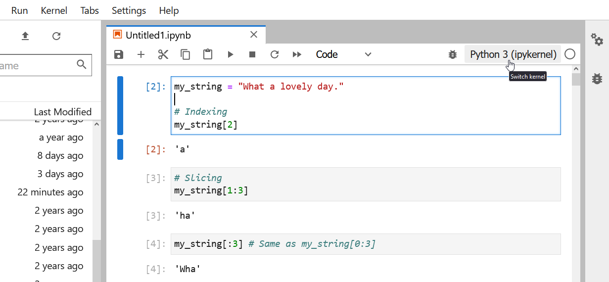
And you should see your conda environments available:
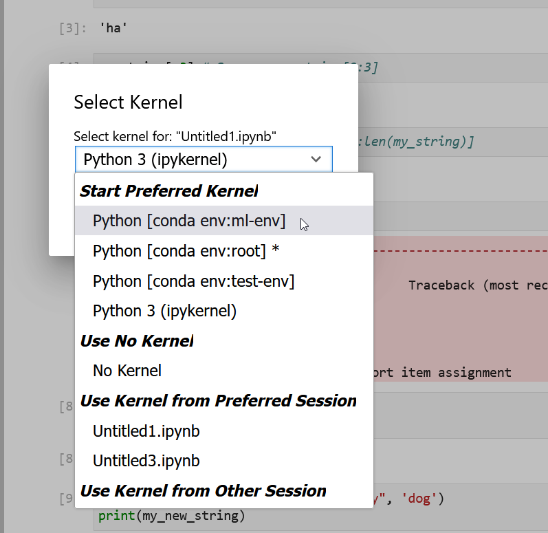
Freezing installed packages
To prevent existing packages from being updating when using the
conda install command, you can use the
--freeze-installed option. This may force Conda to install
older versions of the requested packages in order to maintain
compatibility with previously installed packages. Using the
--freeze-installed option does not prevent additional
dependency packages from being installed.
Where do Conda environments live?
Environments created with conda, by default, live in the
envs/ folder of your miniconda3 (or
anaconda3) directory the absolute path to which will look
something the following: /Users/$USERNAME/miniconda3/envs
or C:\Users\$USERNAME\Anaconda3.
Running ls (linux) / dir (Windows) on your
anaconda envs/ directory will list out the directories
containing the existing Conda environments.
How do I specify a location for a Conda environment?
You can control where a Conda environment lives by providing a path
to a target directory when creating the environment. For example to
following command will create a new environment in a sub-directory of
the current working directory called env.
You activate an environment created with a prefix using the same command used to activate environments created by name.
It is often a good idea to specify a path to a sub-directory of your project directory when creating an environment. Why?
- Makes it easy to tell if your project utilizes an isolated environment by including the environment as a sub-directory.
- Makes your project more self-contained as everything including the required software is contained in a single project directory.
An additional benefit of creating your project’s environment inside a
sub-directory is that you can then use the same name for all your
environments; if you keep all of your environments in your
~/miniconda3/env/ folder, you’ll have to give each of them
a different name.
Listing existing environments
Now that you have created a number of Conda environments on your
local machine you have probably forgotten the names of all of the
environments and exactly where they live. Fortunately, there is a
conda command to list all of your existing environments
together with their locations.
Listing the contents of an environment
In addition to forgetting names and locations of Conda environments,
at some point you will probably forget exactly what has been installed
in a particular Conda environment. Again, there is a conda
command for listing the contents on an environment. To list the contents
of the basic-scipy-env that you created above, run the
following command.
If you created your Conda environment using the --prefix
option to install packages into a particular directory, then you will
need to use that prefix in order for conda to locate the
environment on your machine.
Listing the contents of a particular environment.
List the packages installed in the machine-learning-env
environment that you created in a previous challenge.
You can list the packages and their versions installed in
machine-learning-env using the conda list
command as follows.
To list the packages and their versions installed in the active
environment leave off the --name or --prefix
option.
Deleting entire environments
Occasionally, you will want to delete an entire environment. Perhaps
you were experimenting with conda commands and you created
an environment you have no intention of using; perhaps you no longer
need an existing environment and just want to get rid of cruft on your
machine. Whatever the reason, the command to delete an environment is
the following.
If you wish to delete and environment that you created with a
--prefix option, then you will need to provide the prefix
again when removing the environment.
Delete an entire environment
Delete the entire “basic-scipy-env” environment.
In order to delete an entire environment you use the
conda remove command as follows.
This command will remove all packages from the named environment
before removing the environment itself. The use of the
--yes flag short-circuits the confirmation prompt (and
should be used with caution).
Content from Dictionaries
Last updated on 2023-04-20 | Edit this page
Overview
Questions
- How is a dictionary defined in Python?
- What are the ways to interact with a dictionary?
- Can a dictionary be nested?
Objectives
- Understanding the structure of a dictionary.
- Accessing data from a dictionary.
- Practising nested dictionaries to deal with complex data.
Key Points
- Dictionaries associate a set of values with a number of keys.
- keys are used to access the values of a dictionary.
- Dictionaries are mutable.
- Nested dictionaries are constructed to organise data in a hierarchical fashion.
- Some of the useful methods to work with dictionaries are: .items(), .get()
Dictionary
One of the most useful built-in tools in Python, dictionaries associate a set of values with a number of keys.
Think of an old fashion, paperback dictionary where we have a range of words with their definitions. The words are the keys, and the definitions are the values that are associated with the keys. A Python dictionary works in the same way.
Consider the following scenario:
Suppose we have a number of protein kinases, and we would like to associate them with their descriptions for future reference.
This is an example of association in arrays. We may visualise this problem as displayed below:
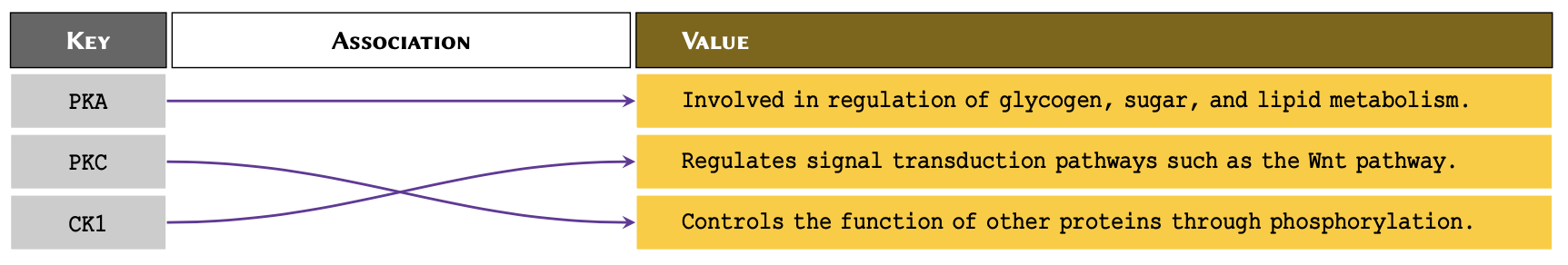
One way to associate the proteins with their definitions would be to use nested arrays. However, it would make it difficult to retrieve the values at a later time. This is because to retrieve the values, we would need to know the index at which a given protein is stored.
Instead of using normal arrays, in such circumstances, we use
associative arrays. The most popular method to create construct
an associative array in Python is to create dictionaries or
dict.
Remember
To implement a dict in Python, we place our entries in
curly bracket, separated using a comma. We separate keys and
values using a colon — e.g. {‘key’: ‘value’}. The combination of
dictionary key and its associating value is known as a
dictionary item.
Note
When constructing a long dict with several
items that span over several lines, it is not necessary to
write one item per line or use indentations for each
item or line. All we must is to write the as {‘key’: ‘value’} in curly brackets and
separate each pair with a comma. However, it is good practice to write
one item per line and use indentations as it makes it
considerably easier to read the code and understand the hierarchy.
We can therefore implement the diagram displayed above in Python as follows:
PYTHON
protein_kinases = {
  'PKA': 'Involved in regulation of glycogen, sugar, and lipid metabolism.',
  'PKC': 'Regulates signal transduction pathways such as the Wnt pathway.',
  'CK1': 'Controls the function of other proteins through phosphorylation.'
  }

print(protein_kinases)
OUTPUT
{'PKA': 'Involved in regulation of glycogen, sugar, and lipid metabolism.', 'PKC': 'Regulates signal transduction pathways such as the Wnt pathway.', 'CK1': 'Controls the function of other proteins through phosphorylation.'}OUTPUT
<class 'dict'>Constructing dictionaries
Use Universal Protein Resource (UniProt) to find the following proteins for humans: - Axin-1 - Rhodopsin
Construct a dictionary for these proteins and the number amino acids for each of them. The keys should represent the name of the protein. Display the result.
Now that we have created a dictionary; we can test whether or not a specific key exists our dictionary:
OUTPUT
TrueOUTPUT
FalseUsing in
Using the proteins dictionary you created in the above
challenge, test to see whether or not a protein called
ERK exists as a key in your dictionary?
Display the result as a Boolean value.
Interacting with a dictionary
We have already learnt that in programming, the more explicit our code, the better it is. Interacting with dictionaries in Python is very easy, coherent, and explicit. This makes them a powerful tool that we can exploit for different purposes.
In lists and tuples, we use indexing and
slicing to retrieve values. In dictionaries, however, we use
keys to do that. Because we can define the keys of a
dictionary ourselves, we no longer have to rely exclusively on numeric
indices.
As a result, we can retrieve the values of a dictionary using their respective keys as follows:
OUTPUT
Controls the function of other proteins through phosphorylation.However, if we attempt to retrieve the value for a
key that does not exist in our dict, a
KeyError will be raised:
ERROR
Error in py_call_impl(callable, dots$args, dots$keywords): KeyError: 'GSK3'

Detailed traceback:
  File "<string>", line 1, in <module>
Dictionary lookup
Implement a dict to represent the following set of
information:
Cystic Fibrosis:
| Full Name | Gene | Type |
|---|---|---|
| Cystic fibrosis transmembrane conductance regulator | CFTR | Membrane Protein |
Using the dictionary you implemented, retrieve and display the gene associated with cystic fibrosis.
Remember
Whilst the values in a dict can be of virtually
any type supported in Python, the keys may only be defined
using immutable types such as string, int, or
tuple. Additionally, the keys in a dictionary must
be unique.
If we attempt to construct a dict using a mutable value
as key, a TypeError will be raised.
For instance, list is a mutable type and therefore
cannot be used as a key:
ERROR
Error in py_call_impl(callable, dots$args, dots$keywords): TypeError: unhashable type: 'list'

Detailed traceback:
  File "<string>", line 1, in <module>
But we can use any immutable type as a key:
OUTPUT
{'ab': 'some value'}OUTPUT
{('a', 'b'): 'some value'}If we define a key more than once, the Python interpreter
constructs the entry in dict using the last instance.
In the following example, we repeat the key ‘pathway’ twice; and as expected, the interpreter only uses the last instance, which in this case represents the value ‘Canonical’:
PYTHON
signal = {
  'name': 'Wnt',
  'pathway': 'Non-Canonical',  # first instance
  'pathway': 'Canonical'  # second instance
  }

print(signal)
{'name': 'Wnt', 'pathway': 'Canonical'}Dictionaries are mutable
Dictionaries are mutable. This means that we can alter their contents. We can make any alterations to a dictionary as long as we use immutable values for the keys.
Suppose we have a dictionary stored in a variable called
protein, holding some information about a specific
protein:
PYTHON
protein = {
  'full name': 'Cystic fibrosis transmembrane conductance regulator',
  'alias': 'CFTR',
  'gene': 'CFTR',
  'type': 'Membrane Protein',
  'common mutations': ['Delta-F508', 'G542X', 'G551D', 'N1303K']
  }
We can add new items to our dictionary or alter the existing ones:
OUTPUT
{'full name': 'Cystic fibrosis transmembrane conductance regulator', 'alias': 'CFTR', 'gene': 'CFTR', 'type': 'Membrane Protein', 'common mutations': ['Delta-F508', 'G542X', 'G551D', 'N1303K'], 'chromosome': 7}
7
We can also alter an existing value in a dictionary using
its key. To do so, we simply access the value using
its key, and treat it as a normal variable; i.e. the same way
we do with members of a list:
OUTPUT
['Delta-F508', 'G542X', 'G551D', 'N1303K']OUTPUT
{'full name': 'Cystic fibrosis transmembrane conductance regulator', 'alias': 'CFTR', 'gene': 'CFTR', 'type': 'Membrane Protein', 'common mutations': ['Delta-F508', 'G542X', 'G551D', 'N1303K', 'W1282X'], 'chromosome': 7}Altering values
Implement the following dictionary:
signal = {'name': 'Wnt', 'pathway': 'Non-Canonical'}}
with respect to signal:
- Correct the value of pathway to “Canonical”;
- Add a new item to the dictionary to represent the receptors for the canonical pathway as “Frizzled” and “LRP”.
Display the altered dictionary as the final result.
Advanced Topic
Displaying an entire dictionary using the print() function
can look a little messy because it is not properly structured. There is,
however, an external library called pprint (Pretty-Print)
that behaves in very similar way to the default print()
function, but structures dictionaries and other arrays in a more
presentable way before displaying them. We do not discuss
``Pretty-Print’’ in this course, but it is a part of Python’s default
library and is therefore installed with Python automatically. To learn
more it, have a read through the official
documentations for the library and review the examples.
Because the keys are immutable, they cannot be altered. However, we can get around this limitation by introducing a new key and assigning the values of the old key to the new one. Once we do that, we can go ahead and remove the old item. The easiest way to remove an item from a dictionary is to use the syntax del:
PYTHON
# Creating a new key and assigning to it the
# values of the old key:
protein['human chromosome'] = protein['chromosome']

print(protein)
OUTPUT
{'full name': 'Cystic fibrosis transmembrane conductance regulator', 'alias': 'CFTR', 'gene': 'CFTR', 'type': 'Membrane Protein', 'common mutations': ['Delta-F508', 'G542X', 'G551D', 'N1303K', 'W1282X'], 'chromosome': 7, 'human chromosome': 7}OUTPUT
{'full name': 'Cystic fibrosis transmembrane conductance regulator', 'alias': 'CFTR', 'gene': 'CFTR', 'type': 'Membrane Protein', 'common mutations': ['Delta-F508', 'G542X', 'G551D', 'N1303K', 'W1282X'], 'human chromosome': 7}We can simplify the above operation using the .pop() method, which removes the specified key from a dictionary and returns any values associated with it:
OUTPUT
{'full name': 'Cystic fibrosis transmembrane conductance regulator', 'alias': 'CFTR', 'gene': 'CFTR', 'type': 'Membrane Protein', 'human chromosome': 7, 'common mutations in caucasians': ['Delta-F508', 'G542X', 'G551D', 'N1303K', 'W1282X']}Reassigning values
Implement a dictionary as:
with respect to signal:
Change the key name from ‘pdb’ to ‘pdb id’ using the .pop() method.
-
Write a code to find out whether the dictionary:
- contains the new key (i.e. ‘pdb id’).
- confirm that it no longer contains the old key (i.e. ‘pdb’)
If both conditions are met, display:
Contains the new key, but not the old one.Otherwise:
Failed to alter the dictionary.Useful methods for dictionary
Now we use some snippets to demonstrate some of the useful
methods associated with dict in Python.
Given a dictionary as:
PYTHON
lac_repressor = {
'pdb id': '1LBI',
'deposit data': '1996-02-17',
'organism': 'Escherichia coli',
'method': 'x-ray',
'resolution': 2.7,
}We can create an array of all items in the dictionary using the .items() method:
OUTPUT
dict_items([('pdb id', '1LBI'), ('deposit data', '1996-02-17'), ('organism', 'Escherichia coli'), ('method', 'x-ray'), ('resolution', 2.7)])The .items() method also returns an array of
tuple members. Each tuple itself consists of 2
members, and is structured as (‘key’: ‘value’). On that account, we
can use its output in the context of a for–loop as
follows:
OUTPUT
pdb id: 1LBI
deposit data: 1996-02-17
organism: Escherichia coli
method: x-ray
resolution: 2.7We learned earlier that if we ask for a key that is not in
the dict, a KeyError will be raised. If we
anticipate this, we can handle it using the .get() method.
The method takes in the key and searches the dictionary to find
it. If found, the associating value is returned. Otherwise, the
method returns None by default. We can also pass a second
value to .get() to replace None in cases that
the requested key does not exist:
OUTPUT
Error in py_call_impl(callable, dots$args, dots$keywords): KeyError: 'gene'
Detailed traceback:
File "<string>", line 1, in <module>OUTPUT
NoneOUTPUT
Not found...Getting multiple values
Implement the lac_repressor dictionary and try to extract the values associated with the following keys:
- organism
- authors
- subunits
- method
If a key does not exist in the dictionary, display No entry instead.
Display the results in the following format:
organism: XXX
authors: XXX PYTHON
lac_repressor = {
'pdb id': '1LBI',
'deposit data': '1996-02-17',
'organism': 'Escherichia coli',
'method': 'x-ray',
'resolution': 2.7,
}
requested_keys = ['organism', 'authors', 'subunits', 'method']
for key in requested_keys:
lac_repressor.get(key, 'No entry')OUTPUT
'Escherichia coli'
'No entry'
'No entry'
'x-ray'
for-loops and dictionaries
Dictionaries and for-loops create a powerful
combination. We can leverage the accessibility of dictionary
values through specific keys that we define ourselves
in a loop to extract data iteratively and repeatedly.
One of the most useful tools that we can create using nothing more
than a for-loop and a dictionary, in only a few lines of
code, is a sequence converter.
Here, we are essentially iterating through a sequence of DNA
nucleotides (sequence),
extracting one character per loop cycle from our string (nucleotide). We then use that
character as a key to retrieve its corresponding value
from our a dictionary (dna2rna). Once we get the
value, we add it to the variable that we initialised using an
empty string outside the scope of our for-loop (rna_sequence). At the end of the
process, the variable rna_sequence will contain a
converted version of our sequence.
PYTHON
sequence = 'CCCATCTTAAGACTTCACAAGACTTGTGAAATCAGACCACTGCTCAATGCGGAACGCCCG'
dna2rna = {"A": "U", "T": "A", "C": "G", "G": "C"}
rna_sequence = str() # Creating an empty string.
for nucleotide in sequence:
rna_sequence += dna2rna[nucleotide]
print('DNA:', sequence)
print('RNA:', rna_sequence)OUTPUT
DNA: CCCATCTTAAGACTTCACAAGACTTGTGAAATCAGACCACTGCTCAATGCGGAACGCCCG
RNA: GGGUAGAAUUCUGAAGUGUUCUGAACACUUUAGUCUGGUGACGAGUUACGCCUUGCGGGCUsing dictionaries as maps
We know that in reverse transcription, RNA nucleotides are converted to their complementary DNA as shown:
| Type | Direction | Nucleotides |
|---|---|---|
| RNA | 5’…’ | U A G C |
| cDNA | 5’…’ | A T C G |
with that in mind:
Use the table to construct a dictionary for reverse transcription, and another dictionary for the conversion of cDNA to DNA.
Using the appropriate dictionary, convert the following mRNA (exon) sequence for human G protein-coupled receptor to its cDNA.
PYTHON
human_gpcr = (
'AUGGAUGUGACUUCCCAAGCCCGGGGCGUGGGCCUGGAGAUGUACCCAGGCACCGCGCAGCCUGCGGCCCCCAACACCACCUC'
'CCCCGAGCUCAACCUGUCCCACCCGCUCCUGGGCACCGCCCUGGCCAAUGGGACAGGUGAGCUCUCGGAGCACCAGCAGUACG'
'UGAUCGGCCUGUUCCUCUCGUGCCUCUACACCAUCUUCCUCUUCCCCAUCGGCUUUGUGGGCAACAUCCUGAUCCUGGUGGUG'
'AACAUCAGCUUCCGCGAGAAGAUGACCAUCCCCGACCUGUACUUCAUCAACCUGGCGGUGGCGGACCUCAUCCUGGUGGCCGA'
'CUCCCUCAUUGAGGUGUUCAACCUGCACGAGCGGUACUACGACAUCGCCGUCCUGUGCACCUUCAUGUCGCUCUUCCUGCAGG'
'UCAACAUGUACAGCAGCGUCUUCUUCCUCACCUGGAUGAGCUUCGACCGCUACAUCGCCCUGGCCAGGGCCAUGCGCUGCAGC'
'CUGUUCCGCACCAAGCACCACGCCCGGCUGAGCUGUGGCCUCAUCUGGAUGGCAUCCGUGUCAGCCACGCUGGUGCCCUUCAC'
'CGCCGUGCACCUGCAGCACACCGACGAGGCCUGCUUCUGUUUCGCGGAUGUCCGGGAGGUGCAGUGGCUCGAGGUCACGCUGG'
'GCUUCAUCGUGCCCUUCGCCAUCAUCGGCCUGUGCUACUCCCUCAUUGUCCGGGUGCUGGUCAGGGCGCACCGGCACCGUGGG'
'CUGCGGCCCCGGCGGCAGAAGGCGCUCCGCAUGAUCCUCGCGGUGGUGCUGGUCUUCUUCGUCUGCUGGCUGCCGGAGAACGU'
'CUUCAUCAGCGUGCACCUCCUGCAGCGGACGCAGCCUGGGGCCGCUCCCUGCAAGCAGUCUUUCCGCCAUGCCCACCCCCUCA'
'CGGGCCACAUUGUCAACCUCACCGCCUUCUCCAACAGCUGCCUAAACCCCCUCAUCUACAGCUUUCUCGGGGAGACCUUCAGG'
'GACAAGCUGAGGCUGUACAUUGAGCAGAAAACAAAUUUGCCGGCCCUGAACCGCUUCUGUCACGCUGCCCUGAAGGCCGUCAU'
'UCCAGACAGCACCGAGCAGUCGGAUGUGAGGUUCAGCAGUGCCGUG'
)Q1:
PYTHON
mrna2cdna = {
'U': 'A',
'A': 'T',
'G': 'C',
'C': 'G'
}
cdna2dna = {
'A': 'T',
'T': 'A',
'C': 'G',
'G': 'C'
}Q2:
OUTPUT
TACCTACACTGAAGGGTTCGGGCCCCGCACCCGGACCTCTACATGGGTCCGTGGCGCGTCGGACGCCGGGGGTTGTGGTGGAGGGGGCTCGAGTTGGACAGGGTGGGCGAGGACCCGTGGCGGGACCGGTTACCCTGTCCACTCGAGAGCCTCGTGGTCGTCATGCACTAGCCGGACAAGGAGAGCACGGAGATGTGGTAGAAGGAGAAGGGGTAGCCGAAACACCCGTTGTAGGACTAGGACCACCACTTGTAGTCGAAGGCGCTCTTCTACTGGTAGGGGCTGGACATGAAGTAGTTGGACCGCCACCGCCTGGAGTAGGACCACCGGCTGAGGGAGTAACTCCACAAGTTGGACGTGCTCGCCATGATGCTGTAGCGGCAGGACACGTGGAAGTACAGCGAGAAGGACGTCCAGTTGTACATGTCGTCGCAGAAGAAGGAGTGGACCTACTCGAAGCTGGCGATGTAGCGGGACCGGTCCCGGTACGCGACGTCGGACAAGGCGTGGTTCGTGGTGCGGGCCGACTCGACACCGGAGTAGACCTACCGTAGGCACAGTCGGTGCGACCACGGGAAGTGGCGGCACGTGGACGTCGTGTGGCTGCTCCGGACGAAGACAAAGCGCCTACAGGCCCTCCACGTCACCGAGCTCCAGTGCGACCCGAAGTAGCACGGGAAGCGGTAGTAGCCGGACACGATGAGGGAGTAACAGGCCCACGACCAGTCCCGCGTGGCCGTGGCACCCGACGCCGGGGCCGCCGTCTTCCGCGAGGCGTACTAGGAGCGCCACCACGACCAGAAGAAGCAGACGACCGACGGCCTCTTGCAGAAGTAGTCGCACGTGGAGGACGTCGCCTGCGTCGGACCCCGGCGAGGGACGTTCGTCAGAAAGGCGGTACGGGTGGGGGAGTGCCCGGTGTAACAGTTGGAGTGGCGGAAGAGGTTGTCGACGGATTTGGGGGAGTAGATGTCGAAAGAGCCCCTCTGGAAGTCCCTGTTCGACTCCGACATGTAACTCGTCTTTTGTTTAAACGGCCGGGACTTGGCGAAGACAGTGCGACGGGACTTCCGGCAGTAAGGTCTGTCGTGGCTCGTCAGCCTACACTCCAAGTCGTCACGGCACContent from Conditionals
Last updated on 2023-04-27 | Edit this page
Overview
Questions
- How can programs do different things for different data?
Objectives
- Correctly write programs that use if and else statements and simple Boolean expressions (without logical operators).
- Trace the execution of unnested conditionals and conditionals inside loops.
Key Points
- Use
ifstatements to control whether or not a block of code is executed. - Conditionals are often used inside loops.
- Use
elseto execute a block of code when anifcondition is not true. - Use
elifto specify additional tests. - Conditions are tested once, in order.
Use if statements to control whether or not a block of
code is executed.
- An
ifstatement (more properly called a conditional statement) controls whether some block of code is executed or not. - Structure is similar to a
forstatement:- First line opens with
ifand ends with a colon - Body containing one or more statements is indented (usually by 4 spaces)
- First line opens with
PYTHON
mass = 3.54
if mass > 3.0:
print(mass, 'is large')
mass = 2.07
if mass > 3.0:
print (mass, 'is large')OUTPUT
3.54 is largeConditionals are often used inside loops.
- Not much point using a conditional when we know the value (as above).
- But useful when we have a collection to process.
OUTPUT
3.54 is large
9.22 is largeUse else to execute a block of code when an
if condition is not true.
-
elsecan be used following anif. - Allows us to specify an alternative to execute when the
ifbranch isn’t taken.
PYTHON
masses = [3.54, 2.07, 9.22, 1.86, 1.71]
for m in masses:
if m > 3.0:
print(m, 'is large')
else:
print(m, 'is small')OUTPUT
3.54 is large
2.07 is small
9.22 is large
1.86 is small
1.71 is smallUse elif to specify additional tests.
- May want to provide several alternative choices, each with its own test.
- Use
elif(short for “else if”) and a condition to specify these. - Always associated with an
if. - Must come before the
else(which is the “catch all”).
PYTHON
masses = [3.54, 2.07, 9.22, 1.86, 1.71]
for m in masses:
if m > 9.0:
print(m, 'is HUGE')
elif m > 3.0:
print(m, 'is large')
else:
print(m, 'is small')OUTPUT
3.54 is large
2.07 is small
9.22 is HUGE
1.86 is small
1.71 is smallConditions are tested once, in order.
- Python steps through the branches of the conditional in order, testing each in turn.
- So ordering matters.
PYTHON
grade = 85
if grade >= 70:
print('grade is C')
elif grade >= 80:
print('grade is B')
elif grade >= 90:
print('grade is A')OUTPUT
grade is C- Does not automatically go back and re-evaluate if values change.
PYTHON
velocity = 10.0
if velocity > 20.0:
print('moving too fast')
else:
print('adjusting velocity')
velocity = 50.0OUTPUT
adjusting velocity- Often use conditionals in a loop to “evolve” the values of variables.
PYTHON
velocity = 10.0
for i in range(5): # execute the loop 5 times
print(i, ':', velocity)
if velocity > 20.0:
print('moving too fast')
velocity = velocity - 5.0
else:
print('moving too slow')
velocity = velocity + 10.0
print('final velocity:', velocity)OUTPUT
0 : 10.0
moving too slow
1 : 20.0
moving too slow
2 : 30.0
moving too fast
3 : 25.0
moving too fast
4 : 20.0
moving too slow
final velocity: 30.0Compound Relations Using and,
or, and Parentheses
Often, you want some combination of things to be true. You can
combine relations within a conditional using and and
or. Continuing the example above, suppose you have
PYTHON
mass = [ 3.54, 2.07, 9.22, 1.86, 1.71]
velocity = [10.00, 20.00, 30.00, 25.00, 20.00]
for i in range(5):
if mass[i] > 5 and velocity[i] > 20:
print("Fast heavy object. Duck!")
elif mass[i] > 2 and mass[i] <= 5 and velocity[i] <= 20:
print("Normal traffic")
elif mass[i] <= 2 and velocity[i] <= 20:
print("Slow light object. Ignore it")
else:
print("Whoa! Something is up with the data. Check it")Just like with arithmetic, you can and should use parentheses
whenever there is possible ambiguity. A good general rule is to
always use parentheses when mixing and and
or in the same condition. That is, instead of:
write one of these:
PYTHON
if (mass[i] <= 2 or mass[i] >= 5) and velocity[i] > 20:
if mass[i] <= 2 or (mass[i] >= 5 and velocity[i] > 20):so it is perfectly clear to a reader (and to Python) what you really mean.
OUTPUT
25.0Trimming Values
Fill in the blanks so that this program creates a new list containing zeroes where the original list’s values were negative and ones where the original list’s values were positive.
PYTHON
original = [-1.5, 0.2, 0.4, 0.0, -1.3, 0.4]
result = ____
for value in original:
if ____:
result.append(0)
else:
____
print(result)OUTPUT
[0, 1, 1, 1, 0, 1]Initializing
Modify this program so that it finds the largest and smallest values in the list no matter what the range of values originally is.
PYTHON
values = [...some test data...]
smallest, largest = None, None
for v in values:
if ____:
smallest, largest = v, v
____:
smallest = min(____, v)
largest = max(____, v)
print(smallest, largest)What are the advantages and disadvantages of using this method to find the range of the data?
PYTHON
values = [-2,1,65,78,-54,-24,100]
smallest, largest = None, None
for v in values:
if smallest is None and largest is None:
smallest, largest = v, v
else:
smallest = min(smallest, v)
largest = max(largest, v)
print(smallest, largest)If you wrote == None instead of is None,
that works too, but Python programmers always write is None
because of the special way None works in the language.
It can be argued that an advantage of using this method would be to
make the code more readable. However, a disadvantage is that this code
is not efficient because within each iteration of the for
loop statement, there are two more loops that run over two numbers each
(the min and max functions). It would be more
efficient to iterate over each number just once:
PYTHON
values = [-2,1,65,78,-54,-24,100]
smallest, largest = None, None
for v in values:
if smallest is None or v < smallest:
smallest = v
if largest is None or v > largest:
largest = v
print(smallest, largest)Now we have one loop, but four comparison tests. There are two ways we could improve it further: either use fewer comparisons in each iteration, or use two loops that each contain only one comparison test. The simplest solution is often the best:
Content from Pandas DataFrames
Last updated on 2023-04-24 | Edit this page
Overview
Questions
- How can I perform statistical analysis of tabular data?
Objectives
- Select individual values from a Pandas dataframe.
- Select entire rows or entire columns from a dataframe.
- Select a subset of both rows and columns from a dataframe in a single operation.
- Select a subset of a dataframe by a single Boolean criterion.
Key Points
- Use
DataFrame.iloc[..., ...]to select values by integer location. - Use
:on its own to mean all columns or all rows. - Select multiple columns or rows using
DataFrame.locand a named slice. - Result of slicing can be used in further operations.
- Use comparisons to select data based on value.
- Select values or NaN using a Boolean mask.
Note about Pandas DataFrames/Series
A DataFrame is a collection of Series; The DataFrame is the way Pandas represents a table, and Series is the data-structure Pandas use to represent a column.
Pandas is built on top of the Numpy library, which in practice means that most of the methods defined for Numpy Arrays apply to Pandas Series/DataFrames.
What makes Pandas so attractive is the powerful interface to access individual records of the table, proper handling of missing values, and relational-databases operations between DataFrames.
The Pandas cheatsheet is a great quick reference for popular dataframe operations.
Data description
We will be using the same data as the previous lesson from Blackmore et al. (2017), The effect of upper-respiratory infection on transcriptomic changes in the CNS.
However, this data file consists only of the expression data in a gene x sample matrix.
Selecting values
To access a value at the position [i,j] of a DataFrame,
we have two options, depending on what is the meaning of i
in use. Remember that a DataFrame provides an index as a way to
identify the rows of the table; a row, then, has a position
inside the table as well as a label, which uniquely identifies
its entry in the DataFrame.
Use DataFrame.iloc[..., ...] to select values by their
(entry) position
- Can specify location by numerical index analogously to 2D version of character selection in strings.
PYTHON
import pandas as pd
url = "https://raw.githubusercontent.com/ccb-hms/workbench-python-workshop/main/episodes/data/expression_matrix.csv"
rnaseq_df = pd.read_csv(url, index_col=0)
print(rnaseq_df.iloc[0, 0])OUTPUT
1230Note how here we used the index of the gene column as opposed to its name. It is often safer to use names instead of indices so that your code is robust to changes in the data layout, but sometimes indices are necessary.
Use DataFrame.loc[..., ...] to select values by their
(entry) label.
- Can specify location by row and/or column name.
OUTPUT
3678Use : on its own to mean all columns or all rows.
- Just like Python’s usual slicing notation.
OUTPUT
GSM2545336 4060
GSM2545337 1616
GSM2545338 1603
GSM2545339 1901
GSM2545340 2171
GSM2545341 3349
GSM2545342 3122
GSM2545343 2008
GSM2545344 2254
GSM2545345 2277
GSM2545346 2985
GSM2545347 3452
GSM2545348 1883
GSM2545349 2014
GSM2545350 2417
GSM2545351 3678
GSM2545352 2920
GSM2545353 2216
GSM2545354 1821
GSM2545362 2842
GSM2545363 2011
GSM2545380 4019
Name: Cyp2d22, dtype: int64- We would get the same result printing
rnaseq_df.loc["Albania"](without a second index).
OUTPUT
gene
AI504432 1136
AW046200 67
AW551984 584
Aamp 4813
Abca12 4
...
Zkscan3 1661
Zranb1 8223
Zranb3 208
Zscan22 433
Zw10 1436
Name: GSM2545351, Length: 1474, dtype: int64- We would get the same result printing
rnaseq_df["GSM2545351"] - We would also get the same result printing
rnaseq_df.GSM2545351(not recommended, because easily confused with.notation for methods)
Select multiple columns or rows using DataFrame.loc and
a named slice.
OUTPUT
GSM2545337 GSM2545338 GSM2545339 GSM2545340 GSM2545341
gene
Nadk 2285 2237 2286 2398 2201
Nap1l5 18287 17176 21950 18655 19160
Nbeal1 2230 2030 2053 1970 1910
Nbl1 2033 1859 1772 2439 3720
Ncf2 76 60 83 73 61
Nck2 683 706 690 644 648
Ncmap 37 40 46 51 138
Ncoa2 5053 4374 4406 4814 5311
Ndufa10 4218 3921 4268 3980 3631
Ndufs1 7042 6672 7413 7090 6943
Neto1 214 183 383 217 164
Nfkbia 740 897 724 873 1000
Nfya 1003 962 944 919 587
Ngb 56 46 135 63 50
Ngef 498 407 587 410 193
Ngp 50 18 131 47 27
Nid1 1521 1395 862 795 673
In the above code, we discover that slicing using
loc is inclusive at both ends, which differs from
slicing using iloc, where slicing
indicates everything up to but not including the final index.
Result of slicing can be used in further operations.
- Usually don’t just print a slice.
- All the statistical operators that work on entire dataframes work the same way on slices.
- E.g., calculate max of a slice.
OUTPUT
GSM2545337 18287
GSM2545338 17176
GSM2545339 21950
GSM2545340 18655
GSM2545341 19160
dtype: int64OUTPUT
GSM2545337 37
GSM2545338 18
GSM2545339 46
GSM2545340 47
GSM2545341 27
dtype: int64Use comparisons to select data based on value.
- Comparison is applied element by element.
- Returns a similarly-shaped dataframe of
TrueandFalse.
PYTHON
# Use a subset of data to keep output readable.
subset = rnaseq_df.iloc[:5, :5]
print('Subset of data:\n', subset)
# Which values were greater than 1000 ?
print('\nWhere are values large?\n', subset > 1000)OUTPUT
Subset of data:
GSM2545336 GSM2545337 GSM2545338 GSM2545339 GSM2545340
gene
AI504432 1230 1085 969 1284 966
AW046200 83 144 129 121 141
AW551984 670 265 202 682 246
Aamp 5621 4049 3797 4375 4095
Abca12 5 8 1 5 3
Where are values large?
GSM2545336 GSM2545337 GSM2545338 GSM2545339 GSM2545340
gene
AI504432 True True False True False
AW046200 False False False False False
AW551984 False False False False False
Aamp True True True True True
Abca12 False False False False FalseSelect values or NaN using a Boolean mask.
- A frame full of Booleans is sometimes called a mask because of how it can be used.
OUTPUT
GSM2545336 GSM2545337 GSM2545338 GSM2545339 GSM2545340
gene
AI504432 1230.0 1085.0 NaN 1284.0 NaN
AW046200 NaN NaN NaN NaN NaN
AW551984 NaN NaN NaN NaN NaN
Aamp 5621.0 4049.0 3797.0 4375.0 4095.0
Abca12 NaN NaN NaN NaN NaN- Get the value where the mask is true, and NaN (Not a Number) where it is false.
- NaNs are ignored by operations like max, min, average, etc. This is different than in other programming languages such as R but makes using masks in this way very useful.
- The behavior towards NaN values can be changed with the
skipnaargument for most pandas methods and functions.
OUTPUT
GSM2545336 GSM2545337 GSM2545338 GSM2545339 GSM2545340
count 2.000000 2.000000 1.0 2.000000 1.0
mean 3425.500000 2567.000000 3797.0 2829.500000 4095.0
std 3104.905876 2095.864499 NaN 2185.667061 NaN
min 1230.000000 1085.000000 3797.0 1284.000000 4095.0
25% 2327.750000 1826.000000 3797.0 2056.750000 4095.0
50% 3425.500000 2567.000000 3797.0 2829.500000 4095.0
75% 4523.250000 3308.000000 3797.0 3602.250000 4095.0
max 5621.000000 4049.000000 3797.0 4375.000000 4095.0Challenge
Why are there still NaNs in this output, when in Pandas
methods like min and max igonre
Nan by default?
We still see NaN because GSM2545337 and GSM2545340 only
have a single value over 1000 in this subset. The standard deviation
(std) is undefined for a single value.
Using multiple dataframes
Pandas vectorizing methods and grouping operations are features that provide users much flexibility to analyse their data.
For instance, let’s say we want to take a look at genes which are highly expressed over time.
To start, let’s take a look at the top genes by mean expression. First we calculate mean expression per gene:
OUTPUT
GSM2545336 2062.191995
GSM2545337 1765.508820
GSM2545338 1667.990502
GSM2545339 1696.120760
GSM2545340 1681.834464
dtype: float64Notice that that this is printing differently than when we printed
Dataframes. Methods which return single values such as
mean by default return a Series instead of a
Dataframe.
OUTPUT
<class 'pandas.core.series.Series'>We can think of a series as a single-column dataframe. Series, since
they only contain a single column, are indexed like lists:
series[start:end].
Now, we can use the sort_values method and look at the
top 10 genes. Note that sort_values when used on a
Dataframe with multiple columns needs a by
argument to specify what column it should be sorted by.
OUTPUT
GSM2545342 1594.116689
GSM2545341 1637.532564
GSM2545338 1667.990502
GSM2545340 1681.834464
GSM2545346 1692.774084
GSM2545339 1696.120760
GSM2545345 1700.161465
GSM2545344 1712.440299
GSM2545337 1765.508820
GSM2545347 1805.396201
dtype: float64Now let’s say we want to do something a bit more complicated. As opposed to getting the top 10 genes across all samples, we want to instead get genes which had the highest absolute expression change from 0 to 4 days.
To do that, we need to load in the sample metadata as a separate dataframe:
PYTHON
url = "https://raw.githubusercontent.com/ccb-hms/workbench-python-workshop/main/episodes/data/metadata.csv"
metadata = pd.read_csv(url, index_col=0)
print(metadata)OUTPUT
organism age sex infection strain time tissue \
sample
GSM2545336 Mus musculus 8 Female InfluenzaA C57BL/6 8 Cerebellum
GSM2545337 Mus musculus 8 Female NonInfected C57BL/6 0 Cerebellum
GSM2545338 Mus musculus 8 Female NonInfected C57BL/6 0 Cerebellum
GSM2545339 Mus musculus 8 Female InfluenzaA C57BL/6 4 Cerebellum
GSM2545340 Mus musculus 8 Male InfluenzaA C57BL/6 4 Cerebellum
GSM2545341 Mus musculus 8 Male InfluenzaA C57BL/6 8 Cerebellum
GSM2545342 Mus musculus 8 Female InfluenzaA C57BL/6 8 Cerebellum
GSM2545343 Mus musculus 8 Male NonInfected C57BL/6 0 Cerebellum
GSM2545344 Mus musculus 8 Female InfluenzaA C57BL/6 4 Cerebellum
GSM2545345 Mus musculus 8 Male InfluenzaA C57BL/6 4 Cerebellum
GSM2545346 Mus musculus 8 Male InfluenzaA C57BL/6 8 Cerebellum
GSM2545347 Mus musculus 8 Male InfluenzaA C57BL/6 8 Cerebellum
GSM2545348 Mus musculus 8 Female NonInfected C57BL/6 0 Cerebellum
GSM2545349 Mus musculus 8 Male NonInfected C57BL/6 0 Cerebellum
GSM2545350 Mus musculus 8 Male InfluenzaA C57BL/6 4 Cerebellum
GSM2545351 Mus musculus 8 Female InfluenzaA C57BL/6 8 Cerebellum
GSM2545352 Mus musculus 8 Female InfluenzaA C57BL/6 4 Cerebellum
GSM2545353 Mus musculus 8 Female NonInfected C57BL/6 0 Cerebellum
GSM2545354 Mus musculus 8 Male NonInfected C57BL/6 0 Cerebellum
GSM2545362 Mus musculus 8 Female InfluenzaA C57BL/6 4 Cerebellum
GSM2545363 Mus musculus 8 Male InfluenzaA C57BL/6 4 Cerebellum
GSM2545380 Mus musculus 8 Female InfluenzaA C57BL/6 8 Cerebellum
mouse
sample
GSM2545336 14
GSM2545337 9
GSM2545338 10
GSM2545339 15
GSM2545340 18
GSM2545341 6
GSM2545342 5
GSM2545343 11
GSM2545344 22
GSM2545345 13
GSM2545346 23
GSM2545347 24
GSM2545348 8
GSM2545349 7
GSM2545350 1
GSM2545351 16
GSM2545352 21
GSM2545353 4
GSM2545354 2
GSM2545362 20
GSM2545363 12
GSM2545380 19
Time is a property of the samples, not of the genes. While we could
add another row to our dataframe indicating time, it makes more sense to
flip our dataframe and add it as a column. We will learn about other
ways to combine dataframes in a future lesson, but for now since
metadata and rnadeq_df have the same index
values we can use the following syntax:
OUTPUT
gene AI504432 AW046200 AW551984 Aamp Abca12 Abcc8 Abhd14a Abi2 \
GSM2545336 1230 83 670 5621 5 2210 490 5627
GSM2545337 1085 144 265 4049 8 1966 495 4383
GSM2545338 969 129 202 3797 1 2181 474 4107
GSM2545339 1284 121 682 4375 5 2362 468 4062
GSM2545340 966 141 246 4095 3 2475 489 4289
gene Abi3bp Abl2 ... Zfp92 Zfp941 Zfyve28 Zgrf1 Zkscan3 Zranb1 \
GSM2545336 807 2392 ... 91 910 3747 644 1732 8837
GSM2545337 1144 2133 ... 46 654 2568 335 1840 5306
GSM2545338 1028 1891 ... 19 560 2635 347 1800 5106
GSM2545339 935 1645 ... 50 782 2623 405 1751 5306
GSM2545340 879 1926 ... 48 696 3140 549 2056 5896
gene Zranb3 Zscan22 Zw10 time
GSM2545336 207 483 1479 8
GSM2545337 179 535 1394 0
GSM2545338 199 533 1279 0
GSM2545339 208 462 1376 4
GSM2545340 184 439 1568 4 Group By: split-apply-combine
We can now group our data by timepoint using
groupby. groupby will combine our data by one
or more columns, and then any summarizing functions we call such as
mean or max will be performed on each
group.
OUTPUT
gene AI504432 AW046200 AW551984 Aamp Abca12 Abcc8 \
time
0 1033.857143 155.285714 238.000000 4602.571429 5.285714 2576.428571
4 1104.500000 152.375000 302.250000 4870.000000 4.250000 2608.625000
8 1014.000000 81.000000 342.285714 4762.571429 4.142857 2291.571429
gene Abhd14a Abi2 Abi3bp Abl2 ... Zfp810 \
time ...
0 591.428571 4880.571429 1174.571429 2170.142857 ... 537.000000
4 546.750000 4902.875000 1060.625000 2077.875000 ... 629.125000
8 432.428571 4945.285714 762.285714 2131.285714 ... 940.428571
gene Zfp92 Zfp941 Zfyve28 Zgrf1 Zkscan3 Zranb1 \
time
0 36.857143 673.857143 3162.428571 398.571429 2105.571429 6014.00
4 43.000000 770.875000 3284.250000 450.125000 1981.500000 6464.25
8 49.000000 765.571429 3649.571429 635.571429 1664.428571 8187.00
gene Zranb3 Zscan22 Zw10
time
0 191.142857 607.428571 1546.285714
4 196.750000 534.500000 1555.125000
8 191.428571 416.428571 1476.428571
[3 rows x 1474 columns]Another way to easily make a Dataframe after using
groupby is to use Pandas’ aggregation function called
agg. Let’s also flip the data back.
OUTPUT
time 0 4 8
gene
AI504432 1033.857143 1104.500 1014.000000
AW046200 155.285714 152.375 81.000000
AW551984 238.000000 302.250 342.285714
Aamp 4602.571429 4870.000 4762.571429
Abca12 5.285714 4.250 4.142857Let’s also make the column names someting more legible using
rename.
PYTHON
time_means = time_means.rename(columns={0: "day_0", 4: "day_4", 8: "day_8"})
print(time_means.head())OUTPUT
time day_0 day_4 day_8
gene
AI504432 1033.857143 1104.500 1014.000000
AW046200 155.285714 152.375 81.000000
AW551984 238.000000 302.250 342.285714
Aamp 4602.571429 4870.000 4762.571429
Abca12 5.285714 4.250 4.142857Now we can calculate the difference between 0 and 4 days:
OUTPUT
time day_0 day_4 day_8 diff_4_0
gene
AI504432 1033.857143 1104.500 1014.000000 70.642857
AW046200 155.285714 152.375 81.000000 -2.910714
AW551984 238.000000 302.250 342.285714 64.250000
Aamp 4602.571429 4870.000 4762.571429 267.428571
Abca12 5.285714 4.250 4.142857 -1.035714And get the top genes. This time we’ll use the nlargest
method instead of sorting:
OUTPUT
time day_0 day_4 day_8 diff_4_0
gene
Glul 48123.285714 55357.500 73947.857143 7234.214286
Sparc 35429.571429 38832.000 56105.714286 3402.428571
Atp1b1 57350.714286 60364.250 59229.000000 3013.535714
Apod 11575.428571 14506.500 31458.142857 2931.071429
Ttyh1 21453.571429 24252.500 30457.428571 2798.928571
Mt1 7601.428571 10112.375 14397.285714 2510.946429
Etnppl 4516.714286 6702.875 8208.142857 2186.160714
Kif5a 36079.571429 37911.750 33410.714286 1832.178571
Pink1 15454.571429 17252.375 23305.285714 1797.803571
Itih3 2467.714286 3976.500 5534.571429 1508.785714Creating new columns
We looked at the absolute expression change when finding top genes, but typically we actually want to look at the log (base 2) fold chage.
The log fold change from x to y can be
calculated as either:
\(log(y) - log(x)\)
or as
\(log(\frac{y}{x})\)
Try calculating the log fold change from 0 to 4 and 0 to 8 days, and
store the result as two new columns in time_means
We will need the log2 function from the
numpy package to do this:
PYTHON
import numpy as np
time_means['logfc_0_4'] = np.log2(time_means['day_4']) - np.log2(time_means['day_0'])
time_means['logfc_0_8'] = np.log2(time_means['day_8']) - np.log2(time_means['day_0'])
print(time_means.head())OUTPUT
time day_0 day_4 day_8 diff_4_0 logfc_0_4 logfc_0_8
gene
AI504432 1033.857143 1104.500 1014.000000 70.642857 0.095357 -0.027979
AW046200 155.285714 152.375 81.000000 -2.910714 -0.027299 -0.938931
AW551984 238.000000 302.250 342.285714 64.250000 0.344781 0.524240
Aamp 4602.571429 4870.000 4762.571429 267.428571 0.081482 0.049301
Abca12 5.285714 4.250 4.142857 -1.035714 -0.314636 -0.351472We can also use the assign dataframe method to create new columns.
PYTHON
time_means = time_means.assign(fc_0_8 = 2**time_means["logfc_0_8"])
print(time_means.iloc[:,5:])OUTPUT
time logfc_0_8 fc_0_8
gene
AI504432 -0.027979 0.980793
AW046200 -0.938931 0.521619
AW551984 0.524240 1.438175
Aamp 0.049301 1.034763
Abca12 -0.351472 0.783784
... ... ...
Zkscan3 -0.339185 0.790488
Zranb1 0.445010 1.361324
Zranb3 0.002155 1.001495
Zscan22 -0.544646 0.685560
Zw10 -0.066695 0.954823
[1474 rows x 2 columns]Extent of Slicing
- Do the two statements below produce the same output?
- Based on this, what rule governs what is included (or not) in numerical slices and named slices in Pandas?
Here’s metadata as a reminder:
organism age sex infection strain time tissue \
sample
GSM2545336 Mus musculus 8 Female InfluenzaA C57BL/6 8 Cerebellum
GSM2545337 Mus musculus 8 Female NonInfected C57BL/6 0 Cerebellum
GSM2545338 Mus musculus 8 Female NonInfected C57BL/6 0 Cerebellum
GSM2545339 Mus musculus 8 Female InfluenzaA C57BL/6 4 Cerebellum
GSM2545340 Mus musculus 8 Male InfluenzaA C57BL/6 4 Cerebellum
mouse
sample
GSM2545336 14
GSM2545337 9
GSM2545338 10
GSM2545339 15
GSM2545340 18 No, they do not produce the same output! The output of the first statement is:
OUTPUT
organism age
sample
GSM2545336 Mus musculus 8
GSM2545337 Mus musculus 8The second statement gives:
OUTPUT
organism age sex
sample
GSM2545336 Mus musculus 8 Female
GSM2545337 Mus musculus 8 Female
GSM2545338 Mus musculus 8 FemaleClearly, the second statement produces an additional column and an
additional row compared to the first statement.
What conclusion can we draw? We see that a numerical slice, 0:2,
omits the final index (i.e. index 2) in the range provided,
while a named slice, ‘GSM2545336’:‘GSM2545338’, includes the
final element.
Let’s go through this piece of code line by line.
This line makes a copy of the metadata dataframe. While we probably
don’t need to make sure deep=True here, as non of our
columns are more complex or compound objects, it never hurts to be
safe.
This line makes a selection: only those rows of first
for which the ‘sex’ column matches ‘Female’ are extracted. Notice how
the Boolean expression inside the brackets,
first['sex'] == 'Female', is used to select only those rows
where the expression is true. Try printing this expression! Can you
print also its individual True/False elements? (hint: first assign the
expression to a variable)
As the syntax suggests, this line drops the row from
second where the label is ‘GSM2545338’. The resulting
dataframe third has one row less than the original
dataframe second.
Again we apply the drop function, but in this case we are dropping
not a row but a whole column. To accomplish this, we need to specify
also the axis parameter (axis is by default set to 0 for
rows, and we change it to 1 for columns).
The final step is to write the data that we have been working on to a
csv file. Pandas makes this easy with the to_csv()
function. The only required argument to the function is the filename.
Note that the file will be written in the directory from which you
started the Jupyter or Python session.
OUTPUT
idxmin:
GSM2545336 Cfhr2
GSM2545337 Cfhr2
GSM2545338 Aox2
GSM2545339 Ascl5
GSM2545340 Ascl5
GSM2545341 BC055402
GSM2545342 Cryga
GSM2545343 Ascl5
GSM2545344 Aox2
GSM2545345 BC055402
GSM2545346 Cpa6
GSM2545347 Cfhr2
GSM2545348 Acmsd
GSM2545349 Fam124b
GSM2545350 Cryga
GSM2545351 Glrp1
GSM2545352 Cfhr2
GSM2545353 Ascl5
GSM2545354 Ascl5
GSM2545362 Cryga
GSM2545363 Adamts19
GSM2545380 Ascl5
dtype: object
idxmax:
GSM2545336 Glul
GSM2545337 Plp1
GSM2545338 Plp1
GSM2545339 Plp1
GSM2545340 Plp1
GSM2545341 Glul
GSM2545342 Glul
GSM2545343 Plp1
GSM2545344 Plp1
GSM2545345 Plp1
GSM2545346 Glul
GSM2545347 Glul
GSM2545348 Plp1
GSM2545349 Plp1
GSM2545350 Plp1
GSM2545351 Glul
GSM2545352 Plp1
GSM2545353 Plp1
GSM2545354 Plp1
GSM2545362 Plp1
GSM2545363 Plp1
GSM2545380 Glul
dtype: objectFor each column in data, idxmin will return
the index value corresponding to each column’s minimum;
idxmax will do accordingly the same for each column’s
maximum value.
You can use these functions whenever you want to get the row index of the minimum/maximum value and not the actual minimum/maximum value.
Many Ways of Access
There are at least two ways of accessing a value or slice of a
DataFrame: by name or index. However, there are many others. For
example, a single column or row can be accessed either as a
DataFrame or a Series object.
Suggest different ways of doing the following operations on a DataFrame:
- Access a single column
- Access a single row
- Access an individual DataFrame element
- Access several columns
- Access several rows
- Access a subset of specific rows and columns
- Access a subset of row and column ranges
1. Access a single column:
PYTHON
# by name
rnaseq_df["col_name"] # as a Series
rnaseq_df[["col_name"]] # as a DataFrame
# by name using .loc
rnaseq_df.T.loc["col_name"] # as a Series
rnaseq_df.T.loc[["col_name"]].T # as a DataFrame
# Dot notation (Series)
rnaseq_df.col_name
# by index (iloc)
rnaseq_df.iloc[:, col_index] # as a Series
rnaseq_df.iloc[:, [col_index]] # as a DataFrame
# using a mask
rnaseq_df.T[rnaseq_df.T.index == "col_name"].T2. Access a single row:
PYTHON
# by name using .loc
rnaseq_df.loc["row_name"] # as a Series
rnaseq_df.loc[["row_name"]] # as a DataFrame
# by name
rnaseq_df.T["row_name"] # as a Series
rnaseq_df.T[["row_name"]].T # as a DataFrame
# by index
rnaseq_df.iloc[row_index] # as a Series
rnaseq_df.iloc[[row_index]] # as a DataFrame
# using mask
rnaseq_df[rnaseq_df.index == "row_name"]3. Access an individual DataFrame element:
PYTHON
# by column/row names
rnaseq_df["column_name"]["row_name"] # as a Series
rnaseq_df[["col_name"]].loc["row_name"] # as a Series
rnaseq_df[["col_name"]].loc[["row_name"]] # as a DataFrame
rnaseq_df.loc["row_name"]["col_name"] # as a value
rnaseq_df.loc[["row_name"]]["col_name"] # as a Series
rnaseq_df.loc[["row_name"]][["col_name"]] # as a DataFrame
rnaseq_df.loc["row_name", "col_name"] # as a value
rnaseq_df.loc[["row_name"], "col_name"] # as a Series. Preserves index. Column name is moved to `.name`.
rnaseq_df.loc["row_name", ["col_name"]] # as a Series. Index is moved to `.name.` Sets index to column name.
rnaseq_df.loc[["row_name"], ["col_name"]] # as a DataFrame (preserves original index and column name)
# by column/row names: Dot notation
rnaseq_df.col_name.row_name
# by column/row indices
rnaseq_df.iloc[row_index, col_index] # as a value
rnaseq_df.iloc[[row_index], col_index] # as a Series. Preserves index. Column name is moved to `.name`
rnaseq_df.iloc[row_index, [col_index]] # as a Series. Index is moved to `.name.` Sets index to column name.
rnaseq_df.iloc[[row_index], [col_index]] # as a DataFrame (preserves original index and column name)
# column name + row index
rnaseq_df["col_name"][row_index]
rnaseq_df.col_name[row_index]
rnaseq_df["col_name"].iloc[row_index]
# column index + row name
rnaseq_df.iloc[:, [col_index]].loc["row_name"] # as a Series
rnaseq_df.iloc[:, [col_index]].loc[["row_name"]] # as a DataFrame
# using masks
rnaseq_df[rnaseq_df.index == "row_name"].T[rnaseq_df.T.index == "col_name"].T4. Access several columns:
PYTHON
# by name
rnaseq_df[["col1", "col2", "col3"]]
rnaseq_df.loc[:, ["col1", "col2", "col3"]]
# by index
rnaseq_df.iloc[:, [col1_index, col2_index, col3_index]]5. Access several rows
PYTHON
# by name
rnaseq_df.loc[["row1", "row2", "row3"]]
# by index
rnaseq_df.iloc[[row1_index, row2_index, row3_index]]6. Access a subset of specific rows and columns
PYTHON
# by names
rnaseq_df.loc[["row1", "row2", "row3"], ["col1", "col2", "col3"]]
# by indices
rnaseq_df.iloc[[row1_index, row2_index, row3_index], [col1_index, col2_index, col3_index]]
# column names + row indices
rnaseq_df[["col1", "col2", "col3"]].iloc[[row1_index, row2_index, row3_index]]
# column indices + row names
rnaseq_df.iloc[:, [col1_index, col2_index, col3_index]].loc[["row1", "row2", "row3"]]7. Access a subset of row and column ranges
PYTHON
# by name
rnaseq_df.loc["row1":"row2", "col1":"col2"]
# by index
rnaseq_df.iloc[row1_index:row2_index, col1_index:col2_index]
# column names + row indices
rnaseq_df.loc[:, "col1_name":"col2_name"].iloc[row1_index:row2_index]
# column indices + row names
rnaseq_df.iloc[:, col1_index:col2_index].loc["row1":"row2"]Content from Writing Functions
Last updated on 2023-04-24 | Edit this page
Overview
Questions
- How can I create my own functions?
- How can I use functions to write better programs?
Objectives
- Explain and identify the difference between function definition and function call.
- Write a function that takes a small, fixed number of arguments and produces a single result.
Key Points
- Break programs down into functions to make them easier to understand.
- Define a function using
defwith a name, parameters, and a block of code. - Defining a function does not run it.
- Arguments in a function call are matched to its defined parameters.
- Functions may return a result to their caller using
return.
Break programs down into functions to make them easier to understand.
- Human beings can only keep a few items in working memory at a time.
- Understand larger/more complicated ideas by understanding and
combining pieces.
- Components in a machine.
- Lemmas when proving theorems.
- Functions serve the same purpose in programs.
- Encapsulate complexity so that we can treat it as a single “thing”.
- Also enables re-use.
- Write one time, use many times.
Define a function using def with a name, parameters,
and a block of code.
- Begin the definition of a new function with
def. - Followed by the name of the function.
- Must obey the same rules as variable names.
- Then parameters in parentheses.
- Empty parentheses if the function doesn’t take any inputs.
- We will discuss this in detail in a moment.
- Then a colon.
- Then an indented block of code.
Defining a function does not run it.
- Defining a function does not run it.
- Like assigning a value to a variable.
- Must call the function to execute the code it contains.
OUTPUT
Hello!Arguments in a function call are matched to its defined parameters.
- Functions are most useful when they can operate on different data.
- Specify parameters when defining a function.
- These become variables when the function is executed.
- Are assigned the arguments in the call (i.e., the values passed to the function).
- If you don’t name the arguments when using them in the call, the arguments will be matched to parameters in the order the parameters are defined in the function.
PYTHON
def print_date(year, month, day):
joined = str(year) + '/' + str(month) + '/' + str(day)
print(joined)
print_date(1871, 3, 19)OUTPUT
1871/3/19Or, we can name the arguments when we call the function, which allows us to specify them in any order and adds clarity to the call site; otherwise as one is reading the code they might forget if the second argument is the month or the day for example.
OUTPUT
1871/3/19- This tweet shared a nice analogy for functions, Twitter:
()contains the ingredients for the function while the body contains the recipe.
Functions may return a result to their caller using
return.
- Use
return ...to give a value back to the caller. - May occur anywhere in the function.
- But functions are easier to understand if
returnoccurs:- At the start to handle special cases.
- At the very end, with a final result.
OUTPUT
average of actual values: 2.6666666666666665OUTPUT
average of empty list: None- Remember: every function returns something.
- A function that doesn’t explicitly
returna value automatically returnsNone.
OUTPUT
1871/3/19
result of call is: NoneIdentifying Syntax Errors
- Read the code below and try to identify what the errors are without running it.
- Run the code and read the error message. Is it a
SyntaxErroror anIndentationError? - Fix the error.
- Repeat steps 2 and 3 until you have fixed all the errors.
OUTPUT
calling <function report at 0x7fd128ff1bf8> 22.5A function call always needs parenthesis, otherwise you get memory address of the function object. So, if we wanted to call the function named report, and give it the value 22.5 to report on, we could have our function call as follows
OUTPUT
calling
pressure is 22.5Order of Operations
-
What’s wrong in this example?
-
After fixing the problem above, explain why running this example code:
gives this output:
OUTPUT
11:37:59 result of call is: None Why is the result of the call
None?
The problem with the example is that the function
print_time()is defined after the call to the function is made. Python doesn’t know how to resolve the nameprint_timesince it hasn’t been defined yet and will raise aNameErrore.g.,NameError: name 'print_time' is not definedThe first line of output
11:37:59is printed by the first line of code,result = print_time(11, 37, 59)that binds the value returned by invokingprint_timeto the variableresult. The second line is from the second print call to print the contents of theresultvariable.print_time()does not explicitlyreturna value, so it automatically returnsNone.
Find the First
Calling by Name
Earlier we saw this function:
PYTHON
def print_date(year, month, day):
joined = str(year) + '/' + str(month) + '/' + str(day)
print(joined)We saw that we can call the function using named arguments, like this:
- What does
print_date(day=1, month=2, year=2003)print? - When have you seen a function call like this before?
- When and why is it useful to call functions this way?
2003/2/1- We saw examples of using named arguments when working with
the pandas library. For example, when reading in a dataset using
data = pd.read_csv('data/gapminder_gdp_europe.csv', index_col='country'), the last argumentindex_colis a named argument.
- Using named arguments can make code more readable since one can see from the function call what name the different arguments have inside the function. It can also reduce the chances of passing arguments in the wrong order, since by using named arguments the order doesn’t matter.
Encapsulation of an If/Print Block
The code below will run on a label-printer for chicken eggs. A digital scale will report a chicken egg mass (in grams) to the computer and then the computer will print a label.
PYTHON
import random
for i in range(10):
# simulating the mass of a chicken egg
# the (random) mass will be 70 +/- 20 grams
mass = 70 + 20.0 * (2.0 * random.random() - 1.0)
print(mass)
# egg sizing machinery prints a label
if mass >= 85:
print("jumbo")
elif mass >= 70:
print("large")
elif mass < 70 and mass >= 55:
print("medium")
else:
print("small")The if-block that classifies the eggs might be useful in other
situations, so to avoid repeating it, we could fold it into a function,
get_egg_label(). Revising the program to use the function
would give us this:
PYTHON
# revised version
import random
for i in range(10):
# simulating the mass of a chicken egg
# the (random) mass will be 70 +/- 20 grams
mass = 70 + 20.0 * (2.0 * random.random() - 1.0)
print(mass, get_egg_label(mass))- Create a function definition for
get_egg_label()that will work with the revised program above. Note that theget_egg_label()function’s return value will be important. Sample output from the above program would be71.23 large. - A dirty egg might have a mass of more than 90 grams, and a spoiled
or broken egg will probably have a mass that’s less than 50 grams.
Modify your
get_egg_label()function to account for these error conditions. Sample output could be25 too light, probably spoiled.
PYTHON
def get_egg_label(mass):
# egg sizing machinery prints a label
egg_label = "Unlabelled"
if mass >= 90:
egg_label = "warning: egg might be dirty"
elif mass >= 85:
egg_label = "jumbo"
elif mass >= 70:
egg_label = "large"
elif mass < 70 and mass >= 55:
egg_label = "medium"
elif mass < 50:
egg_label = "too light, probably spoiled"
else:
egg_label = "small"
return egg_labelSimulating a dynamical system
In mathematics, a dynamical system is a system in which a function describes the time dependence of a point in a geometrical space. A canonical example of a dynamical system is the logistic map, a growth model that computes a new population density (between 0 and 1) based on the current density. In the model, time takes discrete values 0, 1, 2, …
-
Define a function called
logistic_mapthat takes two inputs:x, representing the current population (at timet), and a parameterr = 1. This function should return a value representing the state of the system (population) at timet + 1, using the mapping function:f(t+1) = r * f(t) * [1 - f(t)] Using a
fororwhileloop, iterate thelogistic_mapfunction defined in part 1, starting from an initial population of 0.5, for a period of timet_final = 10. Store the intermediate results in a list so that after the loop terminates you have accumulated a sequence of values representing the state of the logistic map at timest = [0,1,...,t_final](11 values in total). Print this list to see the evolution of the population.Encapsulate the logic of your loop into a function called
iteratethat takes the initial population as its first input, the parametert_finalas its second input and the parameterras its third input. The function should return the list of values representing the state of the logistic map at timest = [0,1,...,t_final]. Run this function for periodst_final = 100and1000and print some of the values. Is the population trending toward a steady state?
-
PYTHON
def iterate(initial_population, t_final, r): population = [initial_population] for t in range(t_final): population.append( logistic_map(population[t], r) ) return population for period in (10, 100, 1000): population = iterate(0.5, period, 1) print(population[-1])The population seems to be approaching zero.OUTPUT
0.06945089389714401 0.009395779870614648 0.0009913908614406382
Using Functions With Conditionals in Pandas
Functions will often contain conditionals. Here is a short example that will indicate which quartile the argument is in based on hand-coded values for the quartile cut points.
PYTHON
def calculate_life_quartile(exp):
if exp < 58.41:
# This observation is in the first quartile
return 1
elif exp >= 58.41 and exp < 67.05:
# This observation is in the second quartile
return 2
elif exp >= 67.05 and exp < 71.70:
# This observation is in the third quartile
return 3
elif exp >= 71.70:
# This observation is in the fourth quartile
return 4
else:
# This observation has bad dataS
return None
calculate_life_quartile(62.5)OUTPUT
2That function would typically be used within a for loop,
but Pandas has a different, more efficient way of doing the same thing,
and that is by applying a function to a dataframe or a portion
of a dataframe. Here is an example, using the definition above.
PYTHON
{'lifeExp_1992': {'Argentina': 71.868, 'Bolivia': 59.957, 'Brazil': 67.057, 'Canada': 77.95, 'Chile': 74.126, 'Colombia': 68.421, 'Costa Rica': 75.713, 'Cuba': 74.414, 'Dominican Republic': 68.457, 'Ecuador': 69.613, 'El Salvador': 66.798, 'Guatemala': 63.373, 'Haiti': 55.089, 'Honduras': 66.399, 'Jamaica': 71.766, 'Mexico': 71.455, 'Nicaragua': 65.843, 'Panama': 72.462, 'Paraguay': 68.225, 'Peru': 66.458, 'Puerto Rico': 73.911, 'Trinidad and Tobago': 69.862, 'United States': 76.09, 'Uruguay': 72.752, 'Venezuela': 71.15}, 'lifeExp_2007': {'Argentina': 75.32, 'Bolivia': 65.554, 'Brazil': 72.39, 'Canada': 80.653, 'Chile': 78.553, 'Colombia': 72.889, 'Costa Rica': 78.782, 'Cuba': 78.273, 'Dominican Republic': 72.235, 'Ecuador': 74.994, 'El Salvador': 71.878, 'Guatemala': 70.259, 'Haiti': 60.916, 'Honduras': 70.198, 'Jamaica': 72.567, 'Mexico': 76.195, 'Nicaragua': 72.899, 'Panama': 75.537, 'Paraguay': 71.752, 'Peru': 71.421, 'Puerto Rico': 78.746, 'Trinidad and Tobago': 69.819, 'United States': 78.242, 'Uruguay': 76.384, 'Venezuela': 73.747}}
data['life_qrtl_1992'] = data['lifeExp_1992'].apply(calculate_life_quartile)
data['life_qrtl_2007'] = data['lifeExp_2007'].apply(calculate_life_quartile)
print(data.iloc[:,2:])There is a lot in that second line, so let’s take it piece by piece.
On the right side of the = we start with
data['lifeExp'], which is the column in the dataframe
called data labeled lifExp. We use the
apply() to do what it says, apply the
calculate_life_quartile to the value of this column for
every row in the dataframe.
Content from Perform Statistical Tests with Scipy
Last updated on 2023-04-27 | Edit this page
Overview
Questions
- How do I use distributions?
- How do I perform statistical tests?
Objectives
- Explore the
scipylibrary. - Define and sample from a distribution.
- Perform a t-test on prepared data.
Key Points
- Scipy is a package with a variety of scientific computing functionality.
- Scipy.stats contains functionality for distributions and statistical tests.
Sci-py is a package with a variety of scientific computing functionality.
SciPy contains a variety of scientific computing modules. It has modules for:
- Integration (scipy.integrate)
- Optimization (scipy.optimize)
- Interpolation (scipy.interpolate)
- Fourier Transforms (scipy.fft)
- Signal Processing (scipy.signal)
- Linear Algebra (scipy.linalg)
- Compressed Sparse Graph Routines (scipy.sparse.csgraph)
- Spatial data structures and algorithms (scipy.spatial)
- Statistics (scipy.stats)
- Multidimensional image processing (scipy.ndimage)
We are only going to look at some of the functionality in
scipy.stats.
Let’s load the module and take a look. Note that the output is not shown here as it is very long.
This is a lot, but we can see that scipy.stats has a
variety of different distributions and functions available for
performing statistics.
Sampling from a distribution
One common reason use a distribution is if we want to generate some random with some kind of structure. Python has a built-in random module which can perform some basic tasks like getting uniform random numbers or shuffling a list, but we need more power to generate more complicated random data.
Distributions in scipy share a set of methods. Some of the important ones are:
-
rvswhich generates random numbers from the distribution. -
pdfwhich gets the probability density function. -
cdfwhich gets the cumulative distribution function. -
statswhich reports various properties of the distribution.
Scipy’s convention is not to create distribution objects, but to pass
parameters as needed into each of these functions. For instance, to
generate 100 normally distributed variables with a mean of 8 and a
standard deviation of 3, we call stats.norm.rvs with those
parameters as loc and scale, respectively.
OUTPUT
array([10.81294892, 9.35960484, 4.13064284, 5.01349956, 11.91542804,
4.40831262, 7.873177 , 2.80427116, 6.93137287, 8.6260419 ,
10.48824661, 4.03472414, 10.01449037, 7.37493941, 6.8729883 ,
8.8247789 , 6.9956787 , 8.2084562 , 9.4272925 , 8.14680254,
1.61100441, 7.14171227, 6.83756279, 13.15778935, 5.87752233,
11.53910465, 9.7899608 , 10.99998659, 5.67069185, 4.43542582,
8.05798467, 4.56883381, 11.2219477 , 9.49666323, 6.09194101,
10.0844057 , 10.3107259 , 5.50683223, 9.97121225, 10.71650187,
7.11465757, 1.81891326, 5.11893454, 5.7602409 , 7.21754014,
8.79988949, 10.37762164, 14.33689265, 6.33571171, 8.06869862,
8.54040514, 7.70807529, 11.35719793, 9.60738274, 6.02998292,
5.68116531, 2.35490176, 10.74582778, 9.8661685 , 13.39578467,
10.04354226, 7.28494967, 10.16128058, -0.59049207, 7.2093563 ,
6.81705905, 5.95187581, 7.51137727, 12.00011092, 10.99417942,
7.84189409, 1.51154885, 5.85094646, 9.24591807, 10.0216898 ,
9.79350275, 7.26730344, 4.94176518, 9.06454997, 2.99129021,
10.8972046 , 12.51642136, 7.31422469, 4.54086114, 4.36204651,
8.33272365, 9.53609612, 7.21441855, 8.58643188, 7.67419071,
10.36948034, 4.405381 , 8.16845496, 2.9752478 , 5.93608394,
4.91781677, 11.60177026, 7.97727669, 8.43215961, 6.97469055])Numpy arrays
Note that the output isn’t a list or pandas object, but is something
called an array. This is an object in the NumPy package. NumPy objects are used by
most scientific packages in Python such as pandas, scikit-learn, and
scipy. It provides a variety of objects and funcionality for performing
fast numeric operations.
Numpy arrays can be indexed and manipulated like Python lists in most instances, but provide extra functionality. We will not be going into more detail about numpy during this workshop.
Performing a t-test with scipy
First, let’s load up a small toy dataset looking at how mouse weight responded to a particular treatment. This data contains 4 columns, the mouse label/number, whether or not it was treated, its sex and its weight.
PYTHON
import pandas as pd
url = "https://raw.githubusercontent.com/ccb-hms/workbench-python-workshop/main/episodes/data/mouse_weight_data.csv"
mouse_df = pd.read_csv(url, index_col="Mouse")
print(mouse_df)OUTPUT
Treated Sex Weight
Mouse
1 True M 22
2 True F 25
3 True M 27
4 True F 23
5 True M 23
6 True F 24
7 True M 26
8 True F 24
9 True M 27
10 True F 27
11 True M 25
12 True F 27
13 True M 26
14 True F 24
15 True M 26
16 False F 25
17 False M 29
18 False F 28
19 False M 27
20 False F 28
21 False M 25
22 False F 23
23 False M 24
24 False F 30
25 False M 24
26 False F 30
27 False M 30
28 False F 28
29 False M 27
30 False F 24We can start by seeing if the mean weight is different between the groups:
PYTHON
treated_mean = mouse_df[mouse_df["Treated"]]["Weight"].mean()
untreated_mean = mouse_df[~mouse_df["Treated"]]["Weight"].mean()
print(f"Treated mean weight: {treated_mean:0.0f}g\nUntreated mean weight: {untreated_mean:0.0f}g")OUTPUT
Treated mean weight: 25g
Untreated mean weight: 27gWe can see that there is a slight different, but it’s unclear if it is real or just a source of randomnes in the data.
The newline character
\n is a special character called the newline character.
It tells Python to go to a new line of text. \n is univeral
to almost all programming languages.
~ in Pandas
Though before we saw that in Python ! is how we indicate
logical NOT, for pandas boolean series we have to use the ~
character to invert every boolean in the series.
Let’s perform a t-test to check for a significant difference. A
one-sample t-test is performed using ttest_1samp. As we
want to compare two groups, we will need to use perform a two-sample
t-test using ttest_ind.
PYTHON
treated_weights = mouse_df[mouse_df["Treated"]]["Weight"]
untreated_weights = mouse_df[~mouse_df["Treated"]]["Weight"]
stats.ttest_ind(treated_weights, untreated_weights)OUTPUT
Ttest_indResult(statistic=-2.2617859482443694, pvalue=0.03166586638057747)Our p-value is about 0.03.
There are a number of arguments we could use to change the test, such as accounting for unequal variance and single-sides tests which can be found here
Challenge
Peform a t-test looking at whether there is a difference by sex as opposed to treatment.
Content from Reshaping Data
Last updated on 2023-04-27 | Edit this page
Overview
Questions
- How can change the shape of my data?
- What is the difference between long and wide data?
Objectives
- Extract substrings of interest.
- Format dynamic strings using f-strings.
- Explore Python’s built-in string functions
Key Points
- Strings can be indexed and sliced.
- Strings cannot be directly altered.
- You can build complex strings based on other variables using f-strings and format.
- Python has a variety of useful built-in string functions.
Wide data and long data
We’ve so far seen our gene expression dataset in two distinct formats which we used for different purposes.
Our original dataset contains a single count value per row, and has all metadata included:
PYTHON
import pandas as pd
url = "https://raw.githubusercontent.com/ccb-hms/workbench-python-workshop/main/episodes/data/rnaseq_reduced.csv"
rnaseq_df = pd.read_csv(url)
print(rnaseq_df)OUTPUT
gene sample expression time
0 Asl GSM2545336 1170 8
1 Apod GSM2545336 36194 8
2 Cyp2d22 GSM2545336 4060 8
3 Klk6 GSM2545336 287 8
4 Fcrls GSM2545336 85 8
... ... ... ... ...
7365 Mgst3 GSM2545340 1563 4
7366 Lrrc52 GSM2545340 2 4
7367 Rxrg GSM2545340 26 4
7368 Lmx1a GSM2545340 81 4
7369 Pbx1 GSM2545340 3805 4
[7370 rows x 4 columns]
Data in this format is referred to as long data.
We also looked at a version of the same data which only contained expression data, where each sample was a column:
PYTHON
url = "https://raw.githubusercontent.com/ccb-hms/workbench-python-workshop/main/episodes/data/expression_matrix.csv"
expression_matrix = pd.read_csv(url, index_col=0)
print(expression_matrix.iloc[:10, :5])OUTPUT
GSM2545336 GSM2545337 GSM2545338 GSM2545339 GSM2545340
gene
AI504432 1230 1085 969 1284 966
AW046200 83 144 129 121 141
AW551984 670 265 202 682 246
Aamp 5621 4049 3797 4375 4095
Abca12 5 8 1 5 3
Abcc8 2210 1966 2181 2362 2475
Abhd14a 490 495 474 468 489
Abi2 5627 4383 4107 4062 4289
Abi3bp 807 1144 1028 935 879
Abl2 2392 2133 1891 1645 1926Data in this format is referred to as wide data.
Each format has its pros and cons, and we often need to switch between the two. Wide data is more human readable, and allows for easy comparision across different samples, such as finding the genes with the highest average expression. However, wide data requires any sample metadata to exist as a separate dataframe. Thus it is much more difficult to examine sample metadata, such as calculating the mean expression at a particular timepoint.
In contrast, long data is considered less human readable. We have to first aggregate our data by gene if we want to do something like calculate average expression. However, we can easily group the data by whatever sample metadata we wish. We will also see in the next session that long data is the preferred format for plotting.
Wide and long data also handle missing data differently. In long
data, and values which don’t exist for a particular sample simply aren’t
rows in the dataset. Thus, our data does not have null
values, but it is harder to tell where data is missing. In wide data,
there is a matrix position for every combination of sample and gene.
Thus, any missing data is shown as a null value. This can
be more difficult to deal with, but makes missing data clear.
Convert from wide to long with melt.
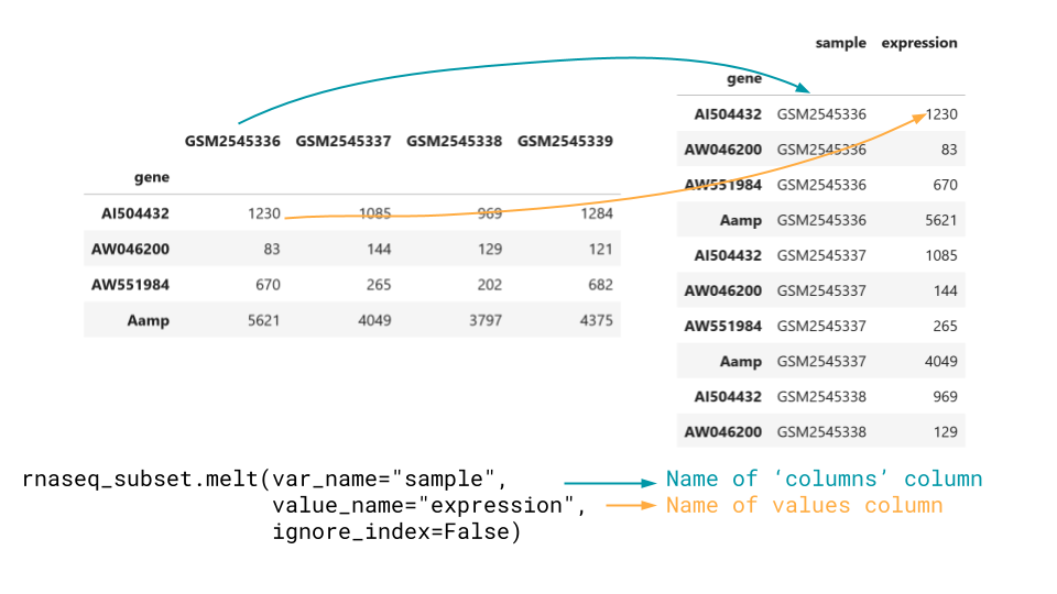
We can convert from wide data to long data using melt.
melt takes in the arguments var_name and
value_name, which are strings that name the two created
columns. We also typically want to set the ignore_index
argument to False, otherwise pandas will drop the dataframe
index.
We could also allow pandas to drop the index, if there is some other
column we want the new rows to be named by, and pass that in instead as
the id_vars argument.
PYTHON
long_data = expression_matrix.melt(var_name="sample", value_name="expression", ignore_index=False)
print(long_data)OUTPUT
sample expression
gene
AI504432 GSM2545336 1230
AW046200 GSM2545336 83
AW551984 GSM2545336 670
Aamp GSM2545336 5621
Abca12 GSM2545336 5
... ... ...
Zkscan3 GSM2545380 1900
Zranb1 GSM2545380 9942
Zranb3 GSM2545380 202
Zscan22 GSM2545380 527
Zw10 GSM2545380 1664
[32428 rows x 2 columns]Convert from long to wide with pivot.
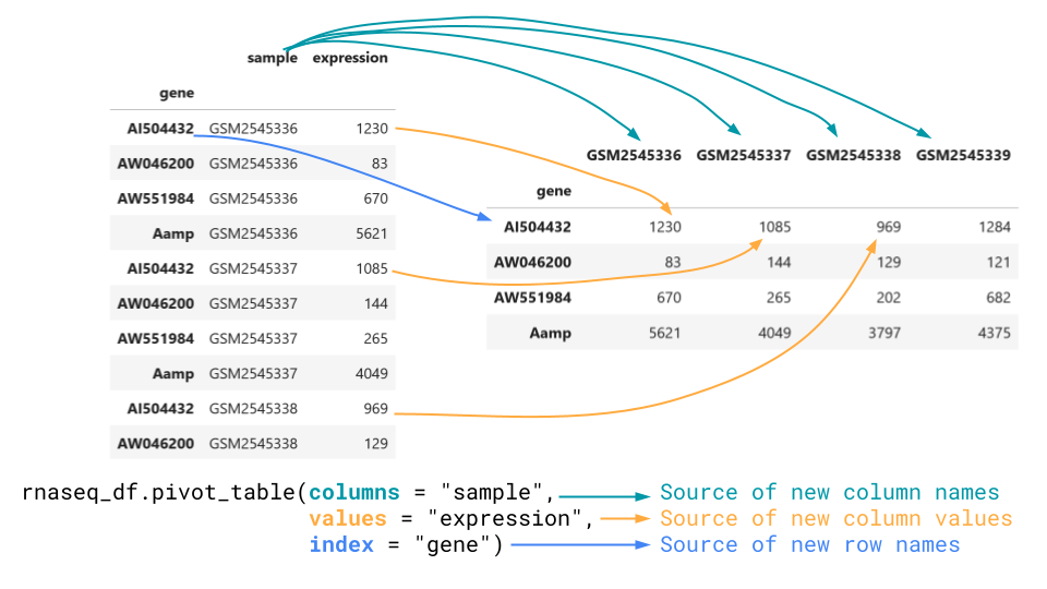
To go the other way, we want to use the pivot_table method.
This method takes in a columns the column to get new
column names from, values, what to populate the matrix
with, and index, what the row names of the wide data should
be.
PYTHON
wide_data = rnaseq_df.pivot_table(columns = "sample", values = "expression", index = "gene")
print(wide_data)OUTPUT
sample GSM2545336 GSM2545337 GSM2545338 GSM2545339 GSM2545340
gene
AI504432 1230 1085 969 1284 966
AW046200 83 144 129 121 141
AW551984 670 265 202 682 246
Aamp 5621 4049 3797 4375 4095
Abca12 5 8 1 5 3
... ... ... ... ... ...
Zkscan3 1732 1840 1800 1751 2056
Zranb1 8837 5306 5106 5306 5896
Zranb3 207 179 199 208 184
Zscan22 483 535 533 462 439
Zw10 1479 1394 1279 1376 1568
[1474 rows x 5 columns]Note that any columns in the dataframe which are not used as values are dropped.
Challenge
Create a dataframe of the rnaseq dataset where each row is a gene and each column is a timepoint instead of a sample. The values in each column should be the mean count across all samples at that timepoint.
Take a look at the aggfunc argument in pivot_table.
What is the default?
Content from Combining Data
Last updated on 2023-04-27 | Edit this page
Overview
Questions
- How can I combine dataframes?
- How do I handle missing or incomplete data mappings?
Objectives
- Determine which kind of combination is desired between two dataframes.
- Combine two dataframes row-wise or column-wise.
- Identify the different types of joins.
Key Points
- Concatenate dataframes to add additional rows.
- Merge/join data frames to add additional columns.
- Change the
onargument to choose what is matched between dataframes when joining. - The different types of joins control how missing data is handled for the left and right dataframes.
There are a variety of ways we might want to combine data when performing a data analysis. We can generally group these into concatenating (sometimes called appending) and merging (sometimes called joining).
We will continue to use the rnaseq dataset:
PYTHON
import pandas as pd
url = "https://raw.githubusercontent.com/ccb-hms/workbench-python-workshop/main/episodes/data/rnaseq.csv"
rnaseq_df = pd.read_csv(url, index_col=0)Concatenate dataframes to add additional rows.
When we want to combine two dataframes by adding one as additional rows, we concatenate them together. This if often the case if our observations are spread out over multiple files. To simulate this, let’s make two miniature versions of `rnaseq_df`` with the first and last 10 rows of the data:
PYTHON
rnaseq_mini = rnaseq_df.loc[:,["sample", "expression"]].head(10)
rnaseq_mini_tail = rnaseq_df.loc[:,["sample", "expression"]].tail(10)
print(rnaseq_mini)
print(rnaseq_mini_tail)OUTPUT
sample expression
gene
Asl GSM2545336 1170
Apod GSM2545336 36194
Cyp2d22 GSM2545336 4060
Klk6 GSM2545336 287
Fcrls GSM2545336 85
Slc2a4 GSM2545336 782
Exd2 GSM2545336 1619
Gjc2 GSM2545336 288
Plp1 GSM2545336 43217
Gnb4 GSM2545336 1071
sample expression
gene
Dusp27 GSM2545380 15
Mael GSM2545380 4
Gm16418 GSM2545380 16
Gm16701 GSM2545380 181
Aldh9a1 GSM2545380 1770
Mgst3 GSM2545380 2151
Lrrc52 GSM2545380 5
Rxrg GSM2545380 49
Lmx1a GSM2545380 72
Pbx1 GSM2545380 4795We can then concatenate the dataframes using the pandas function
concat.
OUTPUT
sample expression
gene
Asl GSM2545336 1170
Apod GSM2545336 36194
Cyp2d22 GSM2545336 4060
Klk6 GSM2545336 287
Fcrls GSM2545336 85
Slc2a4 GSM2545336 782
Exd2 GSM2545336 1619
Gjc2 GSM2545336 288
Plp1 GSM2545336 43217
Gnb4 GSM2545336 1071
Dusp27 GSM2545380 15
Mael GSM2545380 4
Gm16418 GSM2545380 16
Gm16701 GSM2545380 181
Aldh9a1 GSM2545380 1770
Mgst3 GSM2545380 2151
Lrrc52 GSM2545380 5
Rxrg GSM2545380 49
Lmx1a GSM2545380 72
Pbx1 GSM2545380 4795We now have 20 rows in our combined dataset, and the same number of
columns. Note that concat is a function of the
pd module, as opposed to a dataframe method. It takes in a
list of dataframes, and outputs a combined dataframe.
If one dataframe has columns which don’t exist in the other, these
values are filled in with NaN.
PYTHON
rnaseq_mini_time = rnaseq_df.loc[:,["sample", "expression","time"]].iloc[10:20,:]
print(rnaseq_mini_time)OUTPUT
sample expression time
gene
Tnc GSM2545336 219 8
Trf GSM2545336 9719 8
Tubb2b GSM2545336 2245 8
Fads1 GSM2545336 6498 8
Lxn GSM2545336 1744 8
Prr18 GSM2545336 1284 8
Cmtm5 GSM2545336 1381 8
Enpp1 GSM2545336 388 8
Clic4 GSM2545336 5795 8
Tm6sf2 GSM2545336 32 8PYTHON
mini_dfs = [rnaseq_mini, rnaseq_mini_time, rnaseq_mini_tail]
combined_df = pd.concat(mini_dfs)
print(combined_df)OUTPUT
sample expression time
gene
Asl GSM2545336 1170 NaN
Apod GSM2545336 36194 NaN
Cyp2d22 GSM2545336 4060 NaN
Klk6 GSM2545336 287 NaN
Fcrls GSM2545336 85 NaN
Slc2a4 GSM2545336 782 NaN
Exd2 GSM2545336 1619 NaN
Gjc2 GSM2545336 288 NaN
Plp1 GSM2545336 43217 NaN
Gnb4 GSM2545336 1071 NaN
Tnc GSM2545336 219 8.0
Trf GSM2545336 9719 8.0
Tubb2b GSM2545336 2245 8.0
Fads1 GSM2545336 6498 8.0
Lxn GSM2545336 1744 8.0
Prr18 GSM2545336 1284 8.0
Cmtm5 GSM2545336 1381 8.0
Enpp1 GSM2545336 388 8.0
Clic4 GSM2545336 5795 8.0
Tm6sf2 GSM2545336 32 8.0
Dusp27 GSM2545380 15 NaN
Mael GSM2545380 4 NaN
Gm16418 GSM2545380 16 NaN
Gm16701 GSM2545380 181 NaN
Aldh9a1 GSM2545380 1770 NaN
Mgst3 GSM2545380 2151 NaN
Lrrc52 GSM2545380 5 NaN
Rxrg GSM2545380 49 NaN
Lmx1a GSM2545380 72 NaN
Pbx1 GSM2545380 4795 NaNMerge or join data frames to add additional columns.
As opposed to concatenating data, we instead might want to add additional columns to a dataframe. We’ve already seen how to add a new column based on a calculation, but often we have some other data table we want to combine.
If we know that the rows are in the same order, we can use the same syntax we use to assign new columns. However, this is often not the case.
PYTHON
# There is an ongoing idelogical debate among developers whether variables like this should be named:
# url1, url2, and url3
# url0, url1, and url2 or
# url, url2, and url3
url1 = "https://raw.githubusercontent.com/ccb-hms/workbench-python-workshop/main/episodes/data/annot1.csv"
url2 = "https://raw.githubusercontent.com/ccb-hms/workbench-python-workshop/main/episodes/data/annot2.csv"
url3 = "https://raw.githubusercontent.com/ccb-hms/workbench-python-workshop/main/episodes/data/annot3.csv"
# Here .sample is being used to shuffle the dataframe rows into a random order
annot1 = pd.read_csv(url1, index_col=0).sample(frac=1)
annot2 = pd.read_csv(url2, index_col=0).sample(frac=1)
annot3 = pd.read_csv(url3, index_col=0).sample(frac=1)
print(annot1)OUTPUT
gene_description
gene
Fcrls Fc receptor-like S, scavenger receptor [Source...
Plp1 proteolipid protein (myelin) 1 [Source:MGI Sym...
Apod apolipoprotein D [Source:MGI Symbol;Acc:MGI:88...
Klk6 kallikrein related-peptidase 6 [Source:MGI Sym...
Gnb4 guanine nucleotide binding protein (G protein)...
Cyp2d22 cytochrome P450, family 2, subfamily d, polype...
Slc2a4 solute carrier family 2 (facilitated glucose t...
Asl argininosuccinate lyase [Source:MGI Symbol;Acc...
Gjc2 gap junction protein, gamma 2 [Source:MGI Symb...
Exd2 exonuclease 3'-5' domain containing 2 [Source:...OUTPUT
sample expression \
gene
Asl GSM2545336 1170
Apod GSM2545336 36194
Cyp2d22 GSM2545336 4060
Klk6 GSM2545336 287
Fcrls GSM2545336 85
Slc2a4 GSM2545336 782
Exd2 GSM2545336 1619
Gjc2 GSM2545336 288
Plp1 GSM2545336 43217
Gnb4 GSM2545336 1071
gene_description
gene
Asl argininosuccinate lyase [Source:MGI Symbol;Acc...
Apod apolipoprotein D [Source:MGI Symbol;Acc:MGI:88...
Cyp2d22 cytochrome P450, family 2, subfamily d, polype...
Klk6 kallikrein related-peptidase 6 [Source:MGI Sym...
Fcrls Fc receptor-like S, scavenger receptor [Source...
Slc2a4 solute carrier family 2 (facilitated glucose t...
Exd2 exonuclease 3'-5' domain containing 2 [Source:...
Gjc2 gap junction protein, gamma 2 [Source:MGI Symb...
Plp1 proteolipid protein (myelin) 1 [Source:MGI Sym...
Gnb4 guanine nucleotide binding protein (G protein)... We have combined the two dataframes to add the
gene_description column. By default, join
looks at the index column of the left and right dataframe, combining
rows when it finds matches. The data used to determine which rows should
be combined between the dataframes is referred to as what is being
joined on, or the keys. Here, we would say we are joining on
the index columns, or the index columns are the keys. The row order and
column order depends on which dataframe is on the left.
OUTPUT
gene_description sample \
gene
Fcrls Fc receptor-like S, scavenger receptor [Source... GSM2545336
Plp1 proteolipid protein (myelin) 1 [Source:MGI Sym... GSM2545336
Apod apolipoprotein D [Source:MGI Symbol;Acc:MGI:88... GSM2545336
Klk6 kallikrein related-peptidase 6 [Source:MGI Sym... GSM2545336
Gnb4 guanine nucleotide binding protein (G protein)... GSM2545336
Cyp2d22 cytochrome P450, family 2, subfamily d, polype... GSM2545336
Slc2a4 solute carrier family 2 (facilitated glucose t... GSM2545336
Asl argininosuccinate lyase [Source:MGI Symbol;Acc... GSM2545336
Gjc2 gap junction protein, gamma 2 [Source:MGI Symb... GSM2545336
Exd2 exonuclease 3'-5' domain containing 2 [Source:... GSM2545336
expression
gene
Fcrls 85
Plp1 43217
Apod 36194
Klk6 287
Gnb4 1071
Cyp2d22 4060
Slc2a4 782
Asl 1170
Gjc2 288
Exd2 1619
And the index columns do not need to have the same name.
OUTPUT
description
external_gene_name
Slc2a4 solute carrier family 2 (facilitated glucose t...
Gnb4 guanine nucleotide binding protein (G protein)...
Fcrls Fc receptor-like S, scavenger receptor [Source...
Gjc2 gap junction protein, gamma 2 [Source:MGI Symb...
Klk6 kallikrein related-peptidase 6 [Source:MGI Sym...
Plp1 proteolipid protein (myelin) 1 [Source:MGI Sym...
Cyp2d22 cytochrome P450, family 2, subfamily d, polype...
Exd2 exonuclease 3'-5' domain containing 2 [Source:...
Apod apolipoprotein D [Source:MGI Symbol;Acc:MGI:88...
Asl argininosuccinate lyase [Source:MGI Symbol;Acc...OUTPUT
sample expression \
gene
Asl GSM2545336 1170
Apod GSM2545336 36194
Cyp2d22 GSM2545336 4060
Klk6 GSM2545336 287
Fcrls GSM2545336 85
Slc2a4 GSM2545336 782
Exd2 GSM2545336 1619
Gjc2 GSM2545336 288
Plp1 GSM2545336 43217
Gnb4 GSM2545336 1071
description
gene
Asl argininosuccinate lyase [Source:MGI Symbol;Acc...
Apod apolipoprotein D [Source:MGI Symbol;Acc:MGI:88...
Cyp2d22 cytochrome P450, family 2, subfamily d, polype...
Klk6 kallikrein related-peptidase 6 [Source:MGI Sym...
Fcrls Fc receptor-like S, scavenger receptor [Source...
Slc2a4 solute carrier family 2 (facilitated glucose t...
Exd2 exonuclease 3'-5' domain containing 2 [Source:...
Gjc2 gap junction protein, gamma 2 [Source:MGI Symb...
Plp1 proteolipid protein (myelin) 1 [Source:MGI Sym...
Gnb4 guanine nucleotide binding protein (G protein)... join by default uses the indices of the dataframes it
combines. To change this, we can use the on parameter. For
instance, let’s say we want to combine our sample metadata back with
rnaseq_mini.
PYTHON
url = "https://raw.githubusercontent.com/ccb-hms/workbench-python-workshop/main/episodes/data/metadata.csv"
metadata = pd.read_csv(url, index_col=0)
print(metadata)OUTPUT
organism age sex infection strain time tissue \
sample
GSM2545336 Mus musculus 8 Female InfluenzaA C57BL/6 8 Cerebellum
GSM2545337 Mus musculus 8 Female NonInfected C57BL/6 0 Cerebellum
GSM2545338 Mus musculus 8 Female NonInfected C57BL/6 0 Cerebellum
GSM2545339 Mus musculus 8 Female InfluenzaA C57BL/6 4 Cerebellum
GSM2545340 Mus musculus 8 Male InfluenzaA C57BL/6 4 Cerebellum
GSM2545341 Mus musculus 8 Male InfluenzaA C57BL/6 8 Cerebellum
GSM2545342 Mus musculus 8 Female InfluenzaA C57BL/6 8 Cerebellum
GSM2545343 Mus musculus 8 Male NonInfected C57BL/6 0 Cerebellum
GSM2545344 Mus musculus 8 Female InfluenzaA C57BL/6 4 Cerebellum
GSM2545345 Mus musculus 8 Male InfluenzaA C57BL/6 4 Cerebellum
GSM2545346 Mus musculus 8 Male InfluenzaA C57BL/6 8 Cerebellum
GSM2545347 Mus musculus 8 Male InfluenzaA C57BL/6 8 Cerebellum
GSM2545348 Mus musculus 8 Female NonInfected C57BL/6 0 Cerebellum
GSM2545349 Mus musculus 8 Male NonInfected C57BL/6 0 Cerebellum
GSM2545350 Mus musculus 8 Male InfluenzaA C57BL/6 4 Cerebellum
GSM2545351 Mus musculus 8 Female InfluenzaA C57BL/6 8 Cerebellum
GSM2545352 Mus musculus 8 Female InfluenzaA C57BL/6 4 Cerebellum
GSM2545353 Mus musculus 8 Female NonInfected C57BL/6 0 Cerebellum
GSM2545354 Mus musculus 8 Male NonInfected C57BL/6 0 Cerebellum
GSM2545362 Mus musculus 8 Female InfluenzaA C57BL/6 4 Cerebellum
GSM2545363 Mus musculus 8 Male InfluenzaA C57BL/6 4 Cerebellum
GSM2545380 Mus musculus 8 Female InfluenzaA C57BL/6 8 Cerebellum
mouse
sample
GSM2545336 14
GSM2545337 9
GSM2545338 10
GSM2545339 15
GSM2545340 18
GSM2545341 6
GSM2545342 5
GSM2545343 11
GSM2545344 22
GSM2545345 13
GSM2545346 23
GSM2545347 24
GSM2545348 8
GSM2545349 7
GSM2545350 1
GSM2545351 16
GSM2545352 21
GSM2545353 4
GSM2545354 2
GSM2545362 20
GSM2545363 12
GSM2545380 19 OUTPUT
sample expression organism age sex infection \
gene
Asl GSM2545336 1170 Mus musculus 8 Female InfluenzaA
Apod GSM2545336 36194 Mus musculus 8 Female InfluenzaA
Cyp2d22 GSM2545336 4060 Mus musculus 8 Female InfluenzaA
Klk6 GSM2545336 287 Mus musculus 8 Female InfluenzaA
Fcrls GSM2545336 85 Mus musculus 8 Female InfluenzaA
Slc2a4 GSM2545336 782 Mus musculus 8 Female InfluenzaA
Exd2 GSM2545336 1619 Mus musculus 8 Female InfluenzaA
Gjc2 GSM2545336 288 Mus musculus 8 Female InfluenzaA
Plp1 GSM2545336 43217 Mus musculus 8 Female InfluenzaA
Gnb4 GSM2545336 1071 Mus musculus 8 Female InfluenzaA
strain time tissue mouse
gene
Asl C57BL/6 8 Cerebellum 14
Apod C57BL/6 8 Cerebellum 14
Cyp2d22 C57BL/6 8 Cerebellum 14
Klk6 C57BL/6 8 Cerebellum 14
Fcrls C57BL/6 8 Cerebellum 14
Slc2a4 C57BL/6 8 Cerebellum 14
Exd2 C57BL/6 8 Cerebellum 14
Gjc2 C57BL/6 8 Cerebellum 14
Plp1 C57BL/6 8 Cerebellum 14
Gnb4 C57BL/6 8 Cerebellum 14 Note that if we want to join on columns between dataframes which have different names we can simply rename the columns we wish to join on. If there is a reason we don’t want to do this, we can instead use the more powerful but harder to use pandas merge function.
Missing and duplicate data
In the above join, there were a few other things going on. The first
is that multiple rows of rnaseq_mini contain the same
sample. Pandas by default will repeat the rows wherever needed when
joining.
The second is that the metadata dataframe contains
samples which are not present in rnaseq_mini. By default,
they were dropped from the dataframe. However, there might be cases
where we want to keep our data. Let’s explore how joining handles
missing data with another example:
OUTPUT
gene_description
gene
mt-Rnr1 mitochondrially encoded 12S rRNA [Source:MGI S...
mt-Rnr2 mitochondrially encoded 16S rRNA [Source:MGI S...
Slc2a4 solute carrier family 2 (facilitated glucose t...
Asl argininosuccinate lyase [Source:MGI Symbol;Acc...
Exd2 exonuclease 3'-5' domain containing 2 [Source:...
Gnb4 guanine nucleotide binding protein (G protein)...
mt-Tl1 mitochondrially encoded tRNA leucine 1 [Source...
Apod apolipoprotein D [Source:MGI Symbol;Acc:MGI:88...
mt-Tv mitochondrially encoded tRNA valine [Source:MG...
Cyp2d22 cytochrome P450, family 2, subfamily d, polype...
mt-Tf mitochondrially encoded tRNA phenylalanine [So...
Fcrls Fc receptor-like S, scavenger receptor [Source...
Gjc2 gap junction protein, gamma 2 [Source:MGI Symb...
Plp1 proteolipid protein (myelin) 1 [Source:MGI Sym...Missing data in joins
What data is missing between annot3 and
rnaseq_mini?
Try joining them. How is this missing data handled?
There are both genes in annot3 but not in
rnaseq_mini, and genes in rnaseq_mini not in
annot3.
When we join, we keep rows from rnaseq_mini with missing data and
drop rows from annot3 with missing data.
OUTPUT
sample expression \
gene
Asl GSM2545336 1170
Apod GSM2545336 36194
Cyp2d22 GSM2545336 4060
Klk6 GSM2545336 287
Fcrls GSM2545336 85
Slc2a4 GSM2545336 782
Exd2 GSM2545336 1619
Gjc2 GSM2545336 288
Plp1 GSM2545336 43217
Gnb4 GSM2545336 1071
gene_description
gene
Asl argininosuccinate lyase [Source:MGI Symbol;Acc...
Apod apolipoprotein D [Source:MGI Symbol;Acc:MGI:88...
Cyp2d22 cytochrome P450, family 2, subfamily d, polype...
Klk6 NaN
Fcrls Fc receptor-like S, scavenger receptor [Source...
Slc2a4 solute carrier family 2 (facilitated glucose t...
Exd2 exonuclease 3'-5' domain containing 2 [Source:...
Gjc2 gap junction protein, gamma 2 [Source:MGI Symb...
Plp1 proteolipid protein (myelin) 1 [Source:MGI Sym...
Gnb4 guanine nucleotide binding protein (G protein)... Types of joins
The reason we see the above behavior is because by default pandas performs a left join.
We can change the type of join performed by changing the
how argument of the join method.
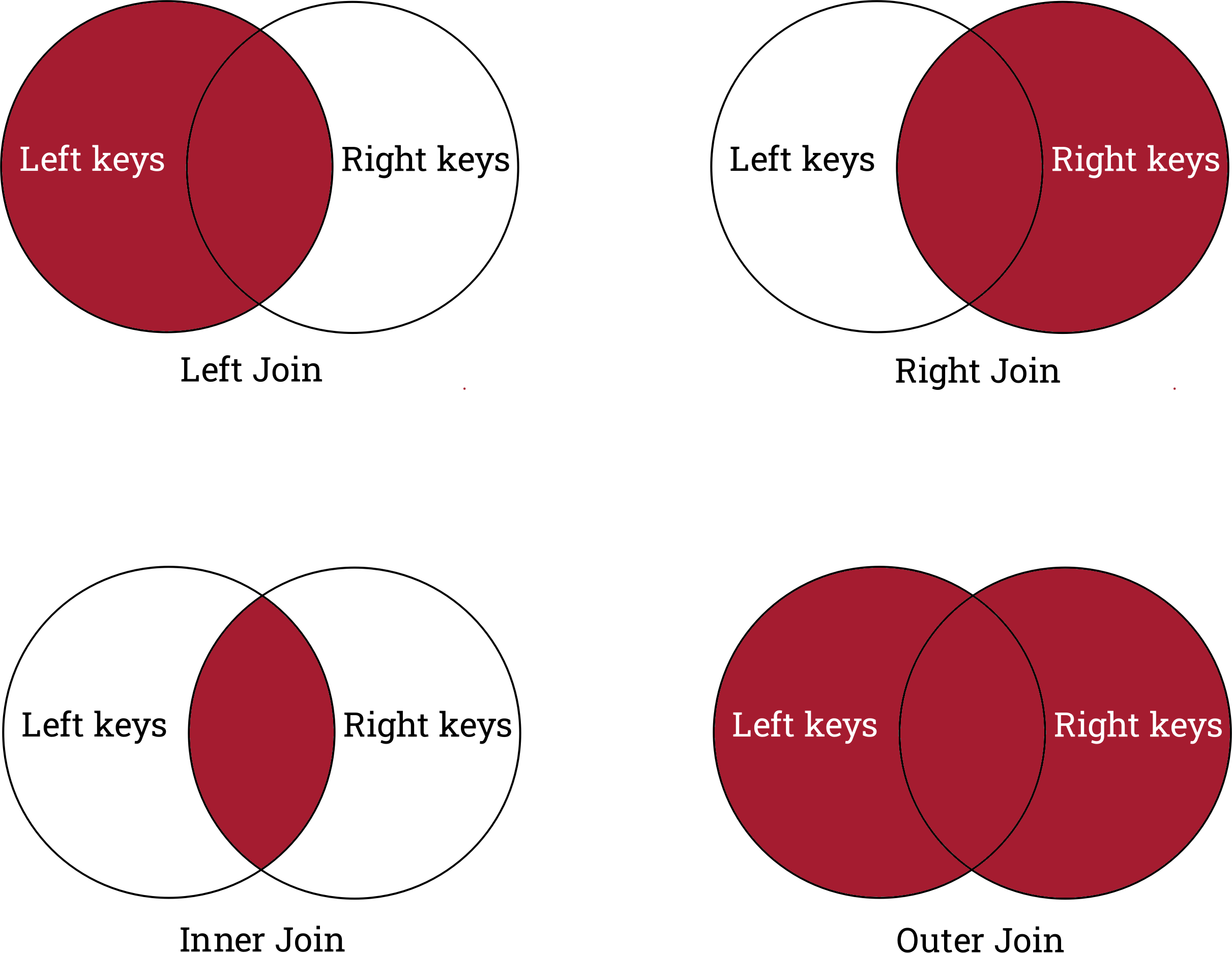
A right join saves all genes in the right dataframe,
but drops and genes unique to rnaseq_mini.
OUTPUT
sample expression \
gene
Plp1 GSM2545336 43217.0
Exd2 GSM2545336 1619.0
Gjc2 GSM2545336 288.0
mt-Rnr2 NaN NaN
Gnb4 GSM2545336 1071.0
mt-Rnr1 NaN NaN
Apod GSM2545336 36194.0
Fcrls GSM2545336 85.0
mt-Tv NaN NaN
mt-Tf NaN NaN
Slc2a4 GSM2545336 782.0
Cyp2d22 GSM2545336 4060.0
mt-Tl1 NaN NaN
Asl GSM2545336 1170.0
gene_description
gene
Plp1 proteolipid protein (myelin) 1 [Source:MGI Sym...
Exd2 exonuclease 3'-5' domain containing 2 [Source:...
Gjc2 gap junction protein, gamma 2 [Source:MGI Symb...
mt-Rnr2 mitochondrially encoded 16S rRNA [Source:MGI S...
Gnb4 guanine nucleotide binding protein (G protein)...
mt-Rnr1 mitochondrially encoded 12S rRNA [Source:MGI S...
Apod apolipoprotein D [Source:MGI Symbol;Acc:MGI:88...
Fcrls Fc receptor-like S, scavenger receptor [Source...
mt-Tv mitochondrially encoded tRNA valine [Source:MG...
mt-Tf mitochondrially encoded tRNA phenylalanine [So...
Slc2a4 solute carrier family 2 (facilitated glucose t...
Cyp2d22 cytochrome P450, family 2, subfamily d, polype...
mt-Tl1 mitochondrially encoded tRNA leucine 1 [Source...
Asl argininosuccinate lyase [Source:MGI Symbol;Acc... An inner join only keeps genes shared by the dataframes, and drops all genes which are only in one dataframe.
OUTPUT
sample expression \
gene
Asl GSM2545336 1170
Apod GSM2545336 36194
Cyp2d22 GSM2545336 4060
Fcrls GSM2545336 85
Slc2a4 GSM2545336 782
Exd2 GSM2545336 1619
Gjc2 GSM2545336 288
Plp1 GSM2545336 43217
Gnb4 GSM2545336 1071
gene_description
gene
Asl argininosuccinate lyase [Source:MGI Symbol;Acc...
Apod apolipoprotein D [Source:MGI Symbol;Acc:MGI:88...
Cyp2d22 cytochrome P450, family 2, subfamily d, polype...
Fcrls Fc receptor-like S, scavenger receptor [Source...
Slc2a4 solute carrier family 2 (facilitated glucose t...
Exd2 exonuclease 3'-5' domain containing 2 [Source:...
Gjc2 gap junction protein, gamma 2 [Source:MGI Symb...
Plp1 proteolipid protein (myelin) 1 [Source:MGI Sym...
Gnb4 guanine nucleotide binding protein (G protein)... Finally, an outer join keeps all genes across both dataframes.
OUTPUT
sample expression \
gene
Apod GSM2545336 36194.0
Asl GSM2545336 1170.0
Cyp2d22 GSM2545336 4060.0
Exd2 GSM2545336 1619.0
Fcrls GSM2545336 85.0
Gjc2 GSM2545336 288.0
Gnb4 GSM2545336 1071.0
Klk6 GSM2545336 287.0
Plp1 GSM2545336 43217.0
Slc2a4 GSM2545336 782.0
mt-Rnr1 NaN NaN
mt-Rnr2 NaN NaN
mt-Tf NaN NaN
mt-Tl1 NaN NaN
mt-Tv NaN NaN
gene_description
gene
Apod apolipoprotein D [Source:MGI Symbol;Acc:MGI:88...
Asl argininosuccinate lyase [Source:MGI Symbol;Acc...
Cyp2d22 cytochrome P450, family 2, subfamily d, polype...
Exd2 exonuclease 3'-5' domain containing 2 [Source:...
Fcrls Fc receptor-like S, scavenger receptor [Source...
Gjc2 gap junction protein, gamma 2 [Source:MGI Symb...
Gnb4 guanine nucleotide binding protein (G protein)...
Klk6 NaN
Plp1 proteolipid protein (myelin) 1 [Source:MGI Sym...
Slc2a4 solute carrier family 2 (facilitated glucose t...
mt-Rnr1 mitochondrially encoded 12S rRNA [Source:MGI S...
mt-Rnr2 mitochondrially encoded 16S rRNA [Source:MGI S...
mt-Tf mitochondrially encoded tRNA phenylalanine [So...
mt-Tl1 mitochondrially encoded tRNA leucine 1 [Source...
mt-Tv mitochondrially encoded tRNA valine [Source:MG... Duplicate column names
One common challenge we encounter when combining datasets from different sources is that they have identical column names.
Imagine that you’ve collected a second set of observations from
samples which are stored in a identically structured file. We can
simulate this by generating some random numbers in a copy of
rnaseq_mini.
PYTHON
new_mini = rnaseq_mini.copy()
new_mini["expression"] = pd.Series(range(50,50000)).sample(int(10), replace=True).array
print(new_mini)Note: as these are pseudo-random numbers your exact values will be different
OUTPUT
sample expression
gene
Asl GSM2545336 48562
Apod GSM2545336 583
Cyp2d22 GSM2545336 39884
Klk6 GSM2545336 6161
Fcrls GSM2545336 10318
Slc2a4 GSM2545336 15991
Exd2 GSM2545336 44471
Gjc2 GSM2545336 40629
Plp1 GSM2545336 23146
Gnb4 GSM2545336 22506Try joining rnaseq_mini and new_mini. What
happens? Take a look at the lsuffix and
rsuffix arguments for join. How can you use
these to improve your joined dataframe?
When we try to join these dataframes we get an error.
ERROR
---------------------------------------------------------------------------
ValueError Traceback (most recent call last)
Cell In[17], line 1
----> 1 rnaseq_mini.join(new_mini)
File ~\anaconda3\envs\ml-env\lib\site-packages\pandas\core\frame.py:9976, in DataFrame.join(self, other, on, how, lsuffix, rsuffix, sort, validate)
9813 def join(
9814 self,
9815 other: DataFrame | Series | list[DataFrame | Series],
(...)
9821 validate: str | None = None,
9822 ) -> DataFrame:
9823 """
9824 Join columns of another DataFrame.
9825
(...)
9974 5 K1 A5 B1
9975 """
-> 9976 return self._join_compat(
9977 other,
9978 on=on,
9979 how=how,
9980 lsuffix=lsuffix,
9981 rsuffix=rsuffix,
9982 sort=sort,
9983 validate=validate,
9984 )
File ~\anaconda3\envs\ml-env\lib\site-packages\pandas\core\frame.py:10015, in DataFrame._join_compat(self, other, on, how, lsuffix, rsuffix, sort, validate)
10005 if how == "cross":
10006 return merge(
10007 self,
10008 other,
(...)
10013 validate=validate,
10014 )
> 10015 return merge(
10016 self,
10017 other,
10018 left_on=on,
10019 how=how,
10020 left_index=on is None,
10021 right_index=True,
10022 suffixes=(lsuffix, rsuffix),
10023 sort=sort,
10024 validate=validate,
10025 )
10026 else:
10027 if on is not None:
File ~\anaconda3\envs\ml-env\lib\site-packages\pandas\core\reshape\merge.py:124, in merge(left, right, how, on, left_on, right_on, left_index, right_index, sort, suffixes, copy, indicator, validate)
93 @Substitution("\nleft : DataFrame or named Series")
94 @Appender(_merge_doc, indents=0)
95 def merge(
(...)
108 validate: str | None = None,
109 ) -> DataFrame:
110 op = _MergeOperation(
111 left,
112 right,
(...)
122 validate=validate,
123 )
--> 124 return op.get_result(copy=copy)
File ~\anaconda3\envs\ml-env\lib\site-packages\pandas\core\reshape\merge.py:775, in _MergeOperation.get_result(self, copy)
771 self.left, self.right = self._indicator_pre_merge(self.left, self.right)
773 join_index, left_indexer, right_indexer = self._get_join_info()
--> 775 result = self._reindex_and_concat(
776 join_index, left_indexer, right_indexer, copy=copy
777 )
778 result = result.__finalize__(self, method=self._merge_type)
780 if self.indicator:
File ~\anaconda3\envs\ml-env\lib\site-packages\pandas\core\reshape\merge.py:729, in _MergeOperation._reindex_and_concat(self, join_index, left_indexer, right_indexer, copy)
726 left = self.left[:]
727 right = self.right[:]
--> 729 llabels, rlabels = _items_overlap_with_suffix(
730 self.left._info_axis, self.right._info_axis, self.suffixes
731 )
733 if left_indexer is not None:
734 # Pinning the index here (and in the right code just below) is not
735 # necessary, but makes the `.take` more performant if we have e.g.
736 # a MultiIndex for left.index.
737 lmgr = left._mgr.reindex_indexer(
738 join_index,
739 left_indexer,
(...)
744 use_na_proxy=True,
745 )
File ~\anaconda3\envs\ml-env\lib\site-packages\pandas\core\reshape\merge.py:2458, in _items_overlap_with_suffix(left, right, suffixes)
2455 lsuffix, rsuffix = suffixes
2457 if not lsuffix and not rsuffix:
-> 2458 raise ValueError(f"columns overlap but no suffix specified: {to_rename}")
2460 def renamer(x, suffix):
2461 """
2462 Rename the left and right indices.
2463
(...)
2474 x : renamed column name
2475 """
ValueError: columns overlap but no suffix specified: Index(['sample', 'expression'], dtype='object')We need to give the datasets suffixes so that there is no column name collision.
OUTPUT
sample_exp1 expression_exp1 sample_exp2 expression_exp2
gene
Asl GSM2545336 1170 GSM2545336 29016
Apod GSM2545336 36194 GSM2545336 46560
Cyp2d22 GSM2545336 4060 GSM2545336 1823
Klk6 GSM2545336 287 GSM2545336 27428
Fcrls GSM2545336 85 GSM2545336 45369
Slc2a4 GSM2545336 782 GSM2545336 31129
Exd2 GSM2545336 1619 GSM2545336 21478
Gjc2 GSM2545336 288 GSM2545336 34747
Plp1 GSM2545336 43217 GSM2545336 46074
Gnb4 GSM2545336 1071 GSM2545336 16370While this works, we now have duplicate sample
columns.
To avoid this, we could either drop the sample column in
one of the dataframes before joining, or use merge to join
on multiple columns and reset the index afterward.
PYTHON
#Option 1: Drop the column
print(rnaseq_mini.join(new_mini.drop('sample',axis=1), lsuffix="_exp1", rsuffix="_exp2"))OUTPUT
sample expression_exp1 expression_exp2
gene
Asl GSM2545336 1170 29016
Apod GSM2545336 36194 46560
Cyp2d22 GSM2545336 4060 1823
Klk6 GSM2545336 287 27428
Fcrls GSM2545336 85 45369
Slc2a4 GSM2545336 782 31129
Exd2 GSM2545336 1619 21478
Gjc2 GSM2545336 288 34747
Plp1 GSM2545336 43217 46074
Gnb4 GSM2545336 1071 16370PYTHON
#Option 2: Merging on gene and sample
print(pd.merge(rnaseq_mini, new_mini, on=["gene","sample"]))OUTPUT
sample expression_x expression_y
gene
Asl GSM2545336 1170 29016
Apod GSM2545336 36194 46560
Cyp2d22 GSM2545336 4060 1823
Klk6 GSM2545336 287 27428
Fcrls GSM2545336 85 45369
Slc2a4 GSM2545336 782 31129
Exd2 GSM2545336 1619 21478
Gjc2 GSM2545336 288 34747
Plp1 GSM2545336 43217 46074
Gnb4 GSM2545336 1071 16370Note that pd.merge does not throw an error when dealing
with duplicate column names, but instead automatically uses the suffixes
_x and _y. We could change these defaults with
the suffixes argument.
Content from Visualizing data with matplotlib and seaborn
Last updated on 2023-04-27 | Edit this page
Overview
Questions
- How can I plot my data?
- How can I save my plot for publishing?
Objectives
- Visualize list-type data using matplotlib.
- Visualize dataframe data with matplotlib and seaborn.
- Customize plot aesthetics.
- Create publication-ready plots for a particular context.
Key Points
-
matplotlibis the most widely used scientific plotting library in Python. - Plot data directly from a Pandas dataframe.
- Select and transform data, then plot it.
- Many styles of plot are available: see the Python Graph Gallery for more options.
- Seaborn extends matplotlib and provides useful defaults and integration with dataframes.
matplotlib is the
most widely used scientific plotting library in Python.
- Commonly use a sub-library called
matplotlib.pyplot. - The Jupyter Notebook will render plots inline by default.
- Simple plots are then (fairly) simple to create.
PYTHON
time = [0, 1, 2, 3]
position = [0, 100, 200, 300]
plt.plot(time, position)
plt.xlabel('Time (hr)')
plt.ylabel('Position (km)')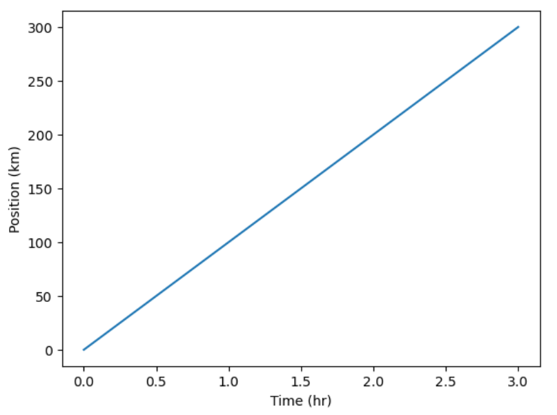
Display All Open Figures
In our Jupyter Notebook example, running the cell should generate the figure directly below the code. The figure is also included in the Notebook document for future viewing. However, other Python environments like an interactive Python session started from a terminal or a Python script executed via the command line require an additional command to display the figure.
Instruct matplotlib to show a figure:
This command can also be used within a Notebook - for instance, to display multiple figures if several are created by a single cell.
Plot data directly from a Pandas dataframe.
- We can also plot Pandas dataframes.
- This implicitly uses
matplotlib.pyplot.
PYTHON
import pandas as pd
url = "https://raw.githubusercontent.com/ccb-hms/workbench-python-workshop/main/episodes/data/rnaseq.csv"
rnaseq_df = pd.read_csv(url, index_col=0)
rnaseq_df.loc[:,'expression'].plot(kind = 'hist')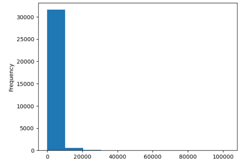
Select and transform data, then plot it.
- By default,
DataFrame.plotplots with the rows as the X axis. - We can transform the data to plot multiple samples.
PYTHON
expression_matrix = rnaseq_df.pivot_table(columns = "time", values = "expression", index="gene")
expression_matrix.plot(kind="box", logy=True)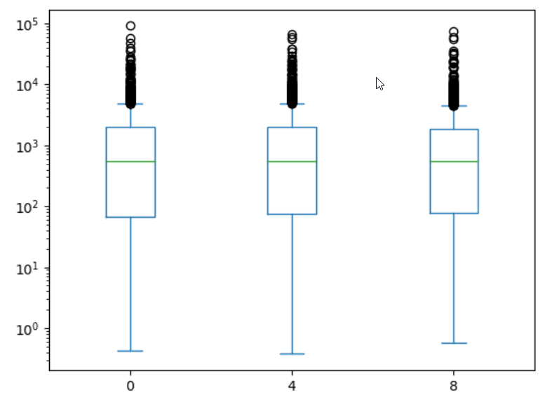
Many plot options are available.
- For example, we can use the
subplotsargument to separate our plot automatically by column.
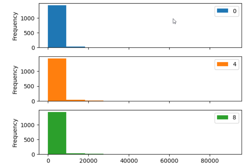
Data can also be plotted by calling the matplotlib
plot function directly.
- The command is
plt.plot(x, y) - The color and format of markers can also be specified as an
additional optional argument e.g.,
b-is a blue line,g--is a green dashed line.
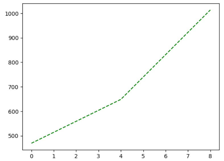
You can plot many sets of data together.
PYTHON
plt.plot(expression_matrix.loc['Asl'], 'g--', label = 'Asl')
plt.plot(expression_matrix.loc['Apod'], 'r-', label = 'Apod')
plt.plot(expression_matrix.loc['Cyp2d22'], 'b-', label = 'Cyp2d22')
plt.plot(expression_matrix.loc['Klk6'], 'b--', label = 'Klk6')
# Create legend.
plt.legend(loc='upper left')
plt.xlabel('Time (days)')
plt.ylabel('Mean Expression')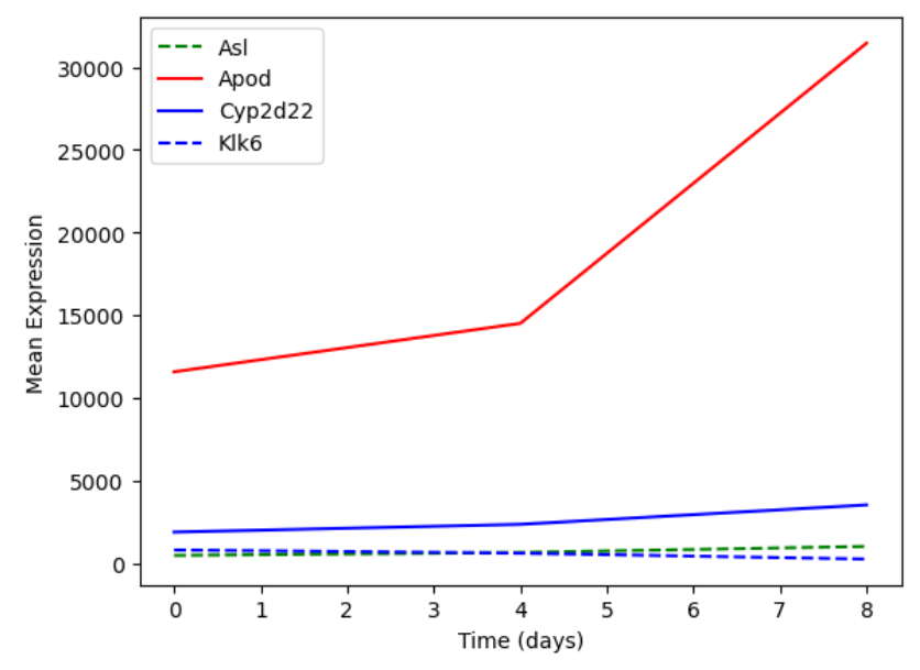
Adding a Legend
Often when plotting multiple datasets on the same figure it is desirable to have a legend describing the data.
This can be done in matplotlib in two stages:
- Provide a label for each dataset in the figure:
PYTHON
plt.plot(expression_matrix.loc['Asl'], 'g--', label = 'Asl')
plt.plot(expression_matrix.loc['Apod'], 'r-', label = 'Apod')- Instruct
matplotlibto create the legend.
By default matplotlib will attempt to place the legend in a suitable
position. If you would rather specify a position this can be done with
the loc= argument, e.g to place the legend in the upper
left corner of the plot, specify loc='upper left'
Seaborn provides more integrated plotting with Pandas and useful defaults
Seaborn is a
plotting library build ontop of matplotlib.pyplot. It
provides higher-level functions for creating high quality data
visualizations, and easily integrates with pandas dataframes.
Let’s see what a boxplot looks like using seaborn.
PYTHON
import seaborn as sns
import numpy as np
#Use seaborn default styling
sns.set_theme()
#Add a log expression column with a pseudocount of 1
rnaseq_df = rnaseq_df.assign(log_exp = np.log2(rnaseq_df["expression"]+1))
sns.boxplot(data = rnaseq_df, x = "time", y = "log_exp")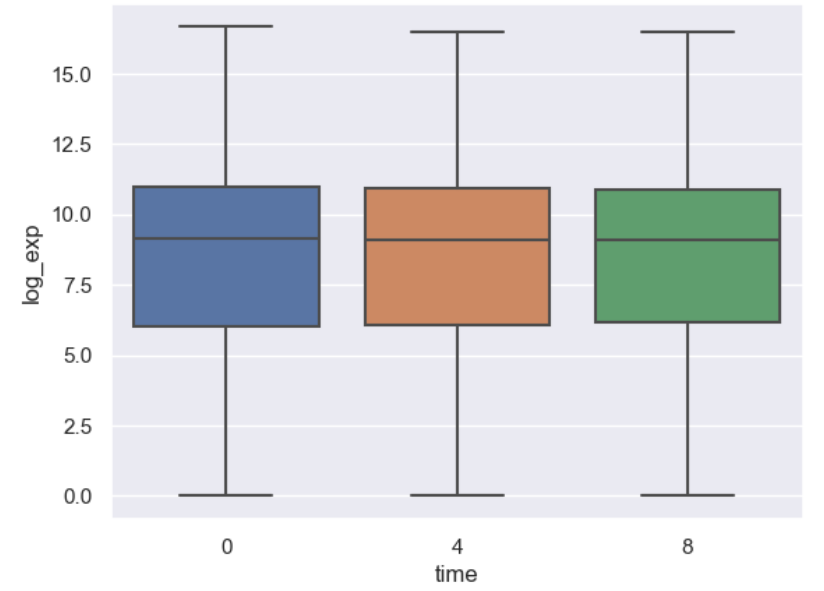
Instead of providing data to x and y directly, with seaborn we
instead give it a dataframe with the data argument, then
tell seaborn which columns of the dataframe we want to be used for each
axis.
Notice that we don’t have to give reshaped data to seaborn, it aggregates our data for us. However, we still have to do more complicated transformations ourselves.
Scenario: log foldchange scatterplot
Imagine we want to compare how different genes behave at different timepoints, and we are expecially interested if genes on any chromosome or of a specific type stnad out. Let’s make a scatterplot of the log-foldchange of our genes step-by-step.
Prepare the data
First, we need to aggregate our data. We could join
expression_matrix with the columns we want from
rnaseq_df, but instead let’s re-pivot our data and bring
gene_biotype and chromosome_name along.
PYTHON
time_matrix = rnaseq_df.pivot_table(columns = "time", values = "log_exp", index=["gene", "chromosome_name", "gene_biotype"])
time_matrix = time_matrix.reset_index(level=["chromosome_name", "gene_biotype"])
print(time_matrix)OUTPUT
time chromosome_name gene_biotype 0 4 8
gene
AI504432 3 lncRNA 10.010544 10.085962 9.974814
AW046200 8 lncRNA 7.275920 7.226188 6.346325
AW551984 9 protein_coding 7.860330 7.264752 8.194396
Aamp 1 protein_coding 12.159714 12.235069 12.198784
Abca12 1 protein_coding 2.509810 2.336441 2.329376
... ... ... ... ... ...
Zkscan3 13 protein_coding 11.031923 10.946440 10.696602
Zranb1 7 protein_coding 12.546820 12.646836 12.984985
Zranb3 1 protein_coding 7.582472 7.611006 7.578124
Zscan22 7 protein_coding 9.239555 9.049392 8.689101
Zw10 9 protein_coding 10.586751 10.598198 10.524456
[1474 rows x 5 columns]Dataframes practice
Starting with time_matrix, add new columns for the log
foldchange from 0 to 4 hours and one with the log foldchange from 0 to 8
hours.
We already have the mean log expression each gene at each timepoint. We need to calculate the foldchange.
PYTHON
# We have to use loc here since our column name is a number
time_matrix["logfc_0_4"] = time_matrix.loc[:,4] - time_matrix.loc[:,0]
time_matrix["logfc_0_8"] = time_matrix.loc[:,8] - time_matrix.loc[:,0]
print(time_matrix)OUTPUT
time chromosome_name gene_biotype 0 4 8 \
gene
AI504432 3 lncRNA 10.010544 10.085962 9.974814
AW046200 8 lncRNA 7.275920 7.226188 6.346325
AW551984 9 protein_coding 7.860330 7.264752 8.194396
Aamp 1 protein_coding 12.159714 12.235069 12.198784
Abca12 1 protein_coding 2.509810 2.336441 2.329376
... ... ... ... ... ...
Zkscan3 13 protein_coding 11.031923 10.946440 10.696602
Zranb1 7 protein_coding 12.546820 12.646836 12.984985
Zranb3 1 protein_coding 7.582472 7.611006 7.578124
Zscan22 7 protein_coding 9.239555 9.049392 8.689101
Zw10 9 protein_coding 10.586751 10.598198 10.524456
time logfc_0_4 logfc_0_8
gene
AI504432 0.075419 -0.035730
AW046200 -0.049732 -0.929596
AW551984 -0.595578 0.334066
Aamp 0.075354 0.039070
Abca12 -0.173369 -0.180433
... ... ...
Zkscan3 -0.085483 -0.335321
Zranb1 0.100015 0.438165
Zranb3 0.028535 -0.004348
Zscan22 -0.190164 -0.550454
Zw10 0.011447 -0.062295
[1474 rows x 7 columns]Note that we could have first calculate foldchange and then log transform it, but performing subtraction is more precise than division in most programming languages, so log transforming first is preferred.
Making an effective scatterplot
Now we can make a scatterplot of the foldchanges.
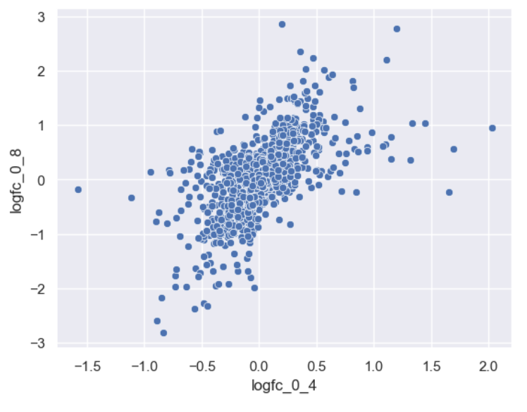
Let’s now improve this plot step-by-step. First we can give the axes more human-readable names than the dataframe’s column names.
PYTHON
sns.scatterplot(data = time_matrix, x = "logfc_0_4", y = "logfc_0_8")
plt.xlabel("0min to 4min (log FC)")
plt.ylabel("0min to 8min (log FC)")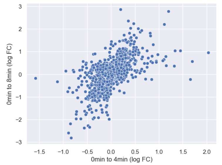
It is difficult to see see the density of genes due to there being so
many points. Lets make the points a little transparent to help with this
by changing their alpha level.
PYTHON
sns.scatterplot(data = time_matrix, x = "logfc_0_4", y = "logfc_0_8", alpha = 0.4)
plt.xlabel("0min to 4min (log FC)")
plt.ylabel("0min to 8min (log FC)")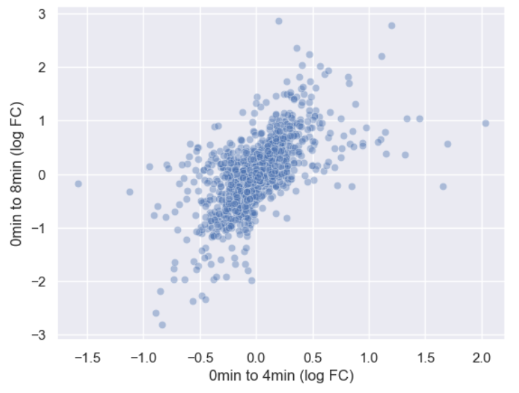
Or we could make the points smaller by adjusting the s
argument.
PYTHON
sns.scatterplot(data = time_matrix, x = "logfc_0_4", y = "logfc_0_8", alpha = 0.6, s=4)
plt.xlabel("0min to 4min (log FC)")
plt.ylabel("0min to 8min (log FC)")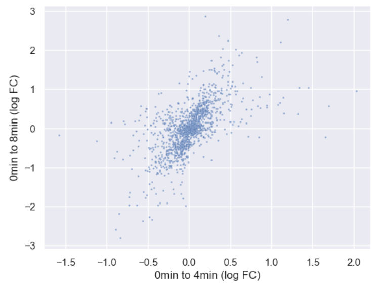
Now let’s incorporate gene_biotype. To do this, we can
set the hue of the scatterplot to the column name. We’re
also going to make some more room for the plot by changing matplotlib’s
rcParams, which are the global plotting settings.
Global plot settings with
rcParams
rcParams is a specialized dictionary used by
matplotlib to store all global plot settings. You can
change rcParams to set things like the
PYTHON
plt.rcParams['figure.figsize'] = [12, 8]
sns.scatterplot(data = time_matrix, x = "logfc_0_4", y = "logfc_0_8", alpha = 0.6, hue="gene_biotype")
plt.xlabel("0min to 4min (log FC)")
plt.ylabel("0min to 8min (log FC)")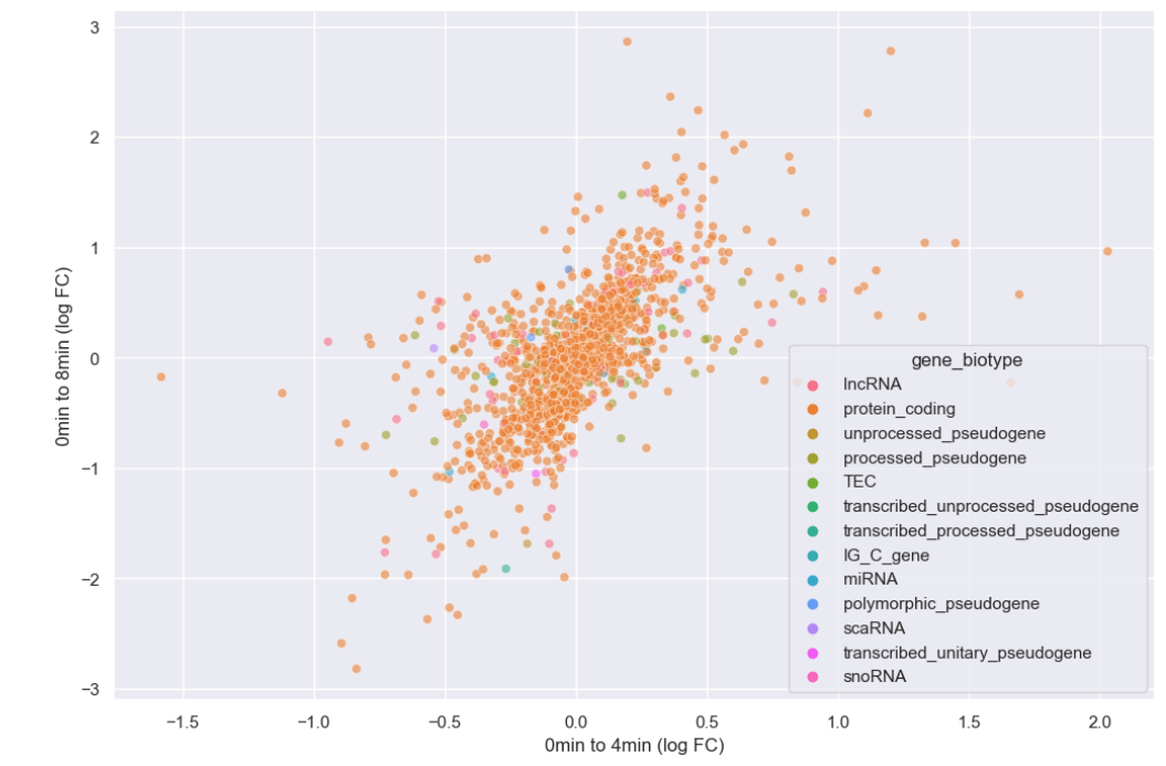
It looks like we overwhelmingly have protein coding genes in the dataset. Instead of plotting every biotype, let’s just plot whether or not the genes are protein coding.
Challenge
Create a new boolean column, is_protein_coding which
specifies whether or not each gene is protein coding.
Make a scatterplot where the style of the points varies
with is_protein_coding.
PYTHON
time_matrix["is_protein_coding"] = time_matrix["gene_biotype"]=="protein_coding"
print(time_matrix)OUTPUT
time chromosome_name gene_biotype 0 4 8 \
gene
AI504432 3 lncRNA 10.010544 10.085962 9.974814
AW046200 8 lncRNA 7.275920 7.226188 6.346325
AW551984 9 protein_coding 7.860330 7.264752 8.194396
Aamp 1 protein_coding 12.159714 12.235069 12.198784
Abca12 1 protein_coding 2.509810 2.336441 2.329376
... ... ... ... ... ...
Zkscan3 13 protein_coding 11.031923 10.946440 10.696602
Zranb1 7 protein_coding 12.546820 12.646836 12.984985
Zranb3 1 protein_coding 7.582472 7.611006 7.578124
Zscan22 7 protein_coding 9.239555 9.049392 8.689101
Zw10 9 protein_coding 10.586751 10.598198 10.524456
time logfc_0_4 logfc_0_8 is_protein_coding
gene
AI504432 0.075419 -0.035730 False
AW046200 -0.049732 -0.929596 False
AW551984 -0.595578 0.334066 True
Aamp 0.075354 0.039070 True
Abca12 -0.173369 -0.180433 True
... ... ... ...
Zkscan3 -0.085483 -0.335321 True
Zranb1 0.100015 0.438165 True
Zranb3 0.028535 -0.004348 True
Zscan22 -0.190164 -0.550454 True
Zw10 0.011447 -0.062295 True
[1474 rows x 8 columns]PYTHON
sns.scatterplot(data = time_matrix, x = "logfc_0_4", y = "logfc_0_8", alpha = 0.6, style="is_protein_coding")
plt.xlabel("0min to 4min (log FC)")
plt.ylabel("0min to 8min (log FC)")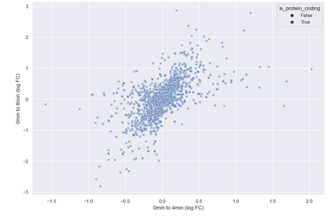
Now that hue is freed up, we can use it to encode for chromosome.
PYTHON
#This hit my personal stylistic limit, so I'm spread the call to multiple lines
sns.scatterplot(data = time_matrix,
x = "logfc_0_4",
y = "logfc_0_8",
alpha = 0.6,
style = "is_protein_coding",
hue = "chromosome_name")
plt.xlabel("0min to 4min (log FC)")
plt.ylabel("0min to 8min (log FC)")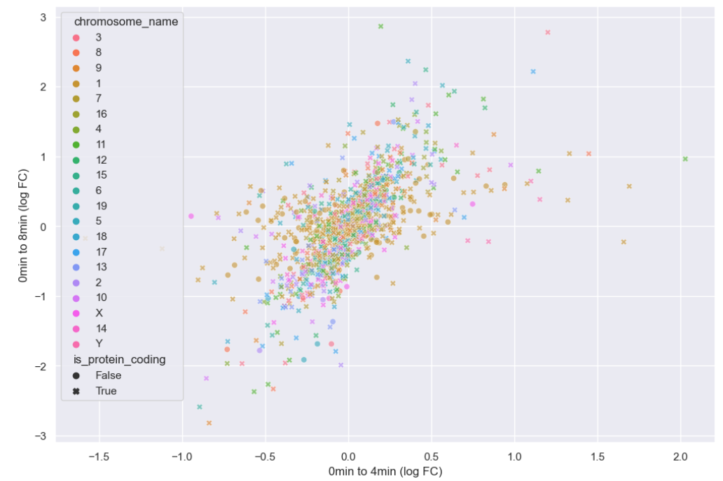
There doesn’t seem to be any interesting pattern. Let’s go back to just plotting whether or not the gene is protein coding, and do a little more to clean up the plot.
PYTHON
# This scales all text in the plot by 150%
sns.set(font_scale = 1.5)
sns.scatterplot(data = time_matrix,
x = "logfc_0_4",
y = "logfc_0_8",
alpha = 0.6,
hue = "is_protein_coding",
#Sets the color pallete to map values to
palette = "mako")
plt.xlabel("0min to 4min (log FC)")
plt.ylabel("0min to 8min (log FC)")
# Set a legend title and give it 2 columns
plt.legend(ncol = 2, title="Is Protein Coding")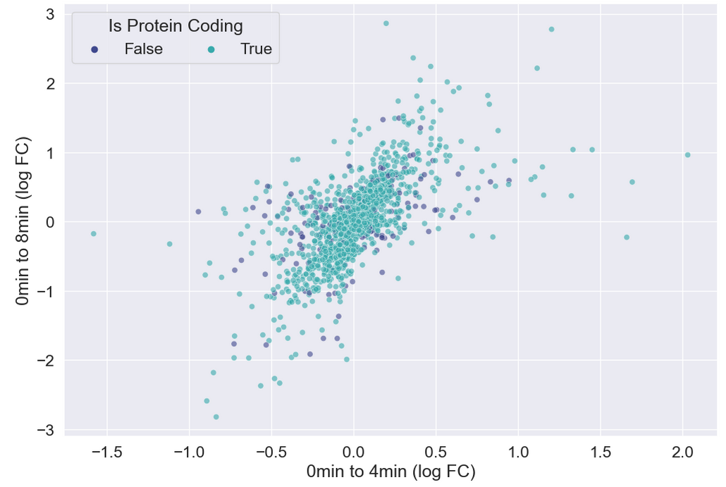
Heatmaps
Seaborn also has great built-in support for heatmaps.
We can make heatmaps using heatmap or
clustermap, depending on if we want our data to be
clustered. Let’s take a look at the correlation matrix for our
samples.
PYTHON
sample_matrix = rnaseq_df.pivot_table(columns = "sample", values = "log_exp", index="gene")
print(sample_matrix.corr())OUTPUT
sample GSM2545336 GSM2545337 GSM2545338 GSM2545339 GSM2545340 \
sample
GSM2545336 1.000000 0.972832 0.970700 0.979381 0.957032
GSM2545337 0.972832 1.000000 0.992230 0.983430 0.972068
GSM2545338 0.970700 0.992230 1.000000 0.981653 0.970098
GSM2545339 0.979381 0.983430 0.981653 1.000000 0.961275
GSM2545340 0.957032 0.972068 0.970098 0.961275 1.000000
GSM2545341 0.957018 0.951554 0.950648 0.940430 0.979411
GSM2545342 0.987712 0.980026 0.978246 0.974903 0.968918
GSM2545343 0.948861 0.971826 0.973301 0.959663 0.988114
GSM2545344 0.973664 0.987626 0.985568 0.980757 0.970084
GSM2545345 0.943748 0.963804 0.963715 0.946226 0.984994
GSM2545346 0.967839 0.961595 0.957958 0.955665 0.984706
GSM2545347 0.958351 0.957363 0.955393 0.944399 0.982981
GSM2545348 0.973558 0.992018 0.991673 0.982984 0.971515
GSM2545349 0.948938 0.970211 0.971276 0.955778 0.988263
GSM2545350 0.952803 0.973764 0.971737 0.960796 0.991229
GSM2545351 0.991921 0.977846 0.973363 0.979936 0.962843
GSM2545352 0.980437 0.989274 0.986909 0.983319 0.974796
GSM2545353 0.974628 0.989940 0.989857 0.982648 0.971325
GSM2545354 0.950621 0.972800 0.972051 0.959123 0.987231
GSM2545362 0.986494 0.981655 0.978767 0.988969 0.962088
GSM2545363 0.936577 0.962115 0.962892 0.940839 0.980774
GSM2545380 0.988869 0.977962 0.975382 0.973683 0.965520
sample GSM2545341 GSM2545342 GSM2545343 GSM2545344 GSM2545345 ... \
sample ...
GSM2545336 0.957018 0.987712 0.948861 0.973664 0.943748 ...
GSM2545337 0.951554 0.980026 0.971826 0.987626 0.963804 ...
GSM2545338 0.950648 0.978246 0.973301 0.985568 0.963715 ...
GSM2545339 0.940430 0.974903 0.959663 0.980757 0.946226 ...
GSM2545340 0.979411 0.968918 0.988114 0.970084 0.984994 ...
GSM2545341 1.000000 0.967231 0.967720 0.958880 0.978091 ...
GSM2545342 0.967231 1.000000 0.959923 0.980462 0.957994 ...
GSM2545343 0.967720 0.959923 1.000000 0.965428 0.983462 ...
GSM2545344 0.958880 0.980462 0.965428 1.000000 0.967708 ...
GSM2545345 0.978091 0.957994 0.983462 0.967708 1.000000 ...
GSM2545346 0.983828 0.973720 0.977478 0.962581 0.976912 ...
GSM2545347 0.986949 0.968972 0.974794 0.962113 0.981518 ...
GSM2545348 0.950961 0.980532 0.974156 0.986710 0.965095 ...
GSM2545349 0.971058 0.960674 0.992085 0.966662 0.986116 ...
GSM2545350 0.973947 0.964523 0.990495 0.970990 0.986146 ...
GSM2545351 0.961638 0.989280 0.953650 0.979976 0.950451 ...
GSM2545352 0.960888 0.985541 0.971954 0.990066 0.968691 ...
GSM2545353 0.952424 0.982904 0.971896 0.989196 0.965436 ...
GSM2545354 0.973524 0.961077 0.988615 0.972600 0.987209 ...
GSM2545362 0.951186 0.982616 0.955145 0.983885 0.946956 ...
GSM2545363 0.970944 0.952557 0.980218 0.965252 0.987553 ...
GSM2545380 0.963521 0.990511 0.957152 0.978371 0.956813 ...
sample GSM2545348 GSM2545349 GSM2545350 GSM2545351 GSM2545352 \
sample
GSM2545336 0.973558 0.948938 0.952803 0.991921 0.980437
GSM2545337 0.992018 0.970211 0.973764 0.977846 0.989274
GSM2545338 0.991673 0.971276 0.971737 0.973363 0.986909
GSM2545339 0.982984 0.955778 0.960796 0.979936 0.983319
GSM2545340 0.971515 0.988263 0.991229 0.962843 0.974796
GSM2545341 0.950961 0.971058 0.973947 0.961638 0.960888
GSM2545342 0.980532 0.960674 0.964523 0.989280 0.985541
GSM2545343 0.974156 0.992085 0.990495 0.953650 0.971954
GSM2545344 0.986710 0.966662 0.970990 0.979976 0.990066
GSM2545345 0.965095 0.986116 0.986146 0.950451 0.968691
GSM2545346 0.960875 0.978673 0.981337 0.971079 0.970621
GSM2545347 0.958524 0.978974 0.980361 0.964883 0.967565
GSM2545348 1.000000 0.971489 0.973997 0.977225 0.990905
GSM2545349 0.971489 1.000000 0.990858 0.954456 0.971922
GSM2545350 0.973997 0.990858 1.000000 0.959045 0.975085
GSM2545351 0.977225 0.954456 0.959045 1.000000 0.983727
GSM2545352 0.990905 0.971922 0.975085 0.983727 1.000000
GSM2545353 0.992297 0.969924 0.972310 0.979291 0.991556
GSM2545354 0.972151 0.990242 0.989228 0.956395 0.972436
GSM2545362 0.980224 0.955712 0.959541 0.988591 0.984683
GSM2545363 0.963226 0.983872 0.982521 0.943499 0.966163
GSM2545380 0.979398 0.956662 0.961779 0.989683 0.985750
sample GSM2545353 GSM2545354 GSM2545362 GSM2545363 GSM2545380
sample
GSM2545336 0.974628 0.950621 0.986494 0.936577 0.988869
GSM2545337 0.989940 0.972800 0.981655 0.962115 0.977962
GSM2545338 0.989857 0.972051 0.978767 0.962892 0.975382
GSM2545339 0.982648 0.959123 0.988969 0.940839 0.973683
GSM2545340 0.971325 0.987231 0.962088 0.980774 0.965520
GSM2545341 0.952424 0.973524 0.951186 0.970944 0.963521
GSM2545342 0.982904 0.961077 0.982616 0.952557 0.990511
GSM2545343 0.971896 0.988615 0.955145 0.980218 0.957152
GSM2545344 0.989196 0.972600 0.983885 0.965252 0.978371
GSM2545345 0.965436 0.987209 0.946956 0.987553 0.956813
GSM2545346 0.963956 0.975386 0.961966 0.967480 0.973104
GSM2545347 0.961118 0.977208 0.952988 0.972364 0.967319
GSM2545348 0.992297 0.972151 0.980224 0.963226 0.979398
GSM2545349 0.969924 0.990242 0.955712 0.983872 0.956662
GSM2545350 0.972310 0.989228 0.959541 0.982521 0.961779
GSM2545351 0.979291 0.956395 0.988591 0.943499 0.989683
GSM2545352 0.991556 0.972436 0.984683 0.966163 0.985750
GSM2545353 1.000000 0.971512 0.980850 0.962497 0.981468
GSM2545354 0.971512 1.000000 0.958851 0.983429 0.957011
GSM2545362 0.980850 0.958851 1.000000 0.942461 0.980664
GSM2545363 0.962497 0.983429 0.942461 1.000000 0.951069
GSM2545380 0.981468 0.957011 0.980664 0.951069 1.000000
[22 rows x 22 columns]We can see the structure of these correlations in a clustered heatmap.
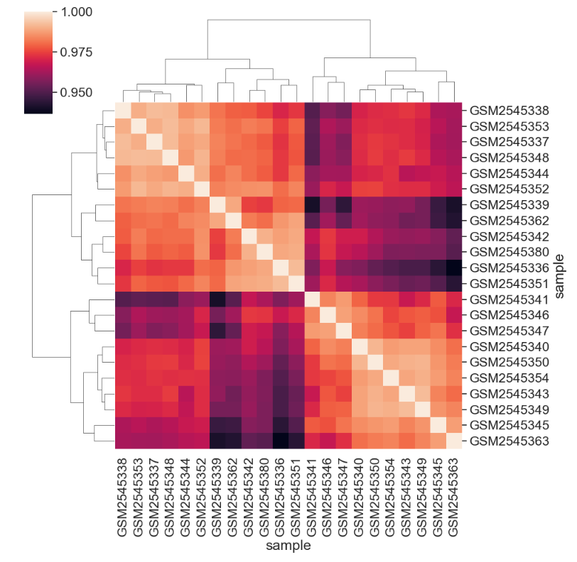
We can change the color mapping.
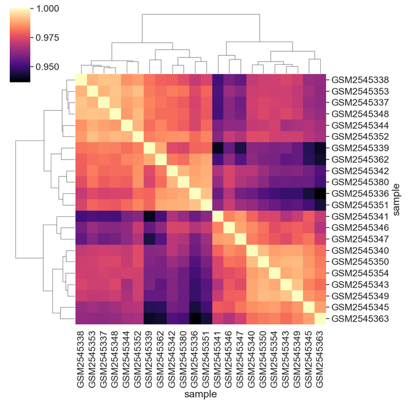
We can add sample information to the plot by changing the index. First we need to get the data.
PYTHON
# We select all of the columns related to the samples we might want to look at, group by sample, then aggregate by the most common value, or mode
sample_data = rnaseq_df[['sample','organism', 'age', 'sex', 'infection',
'strain', 'time', 'tissue', 'mouse']].groupby('sample').agg(pd.Series.mode)
print(sample_data)OUTPUT
organism age sex infection strain time tissue mouse
sample
GSM2545336 Mus musculus 8 Female InfluenzaA C57BL/6 8 Cerebellum 14
GSM2545337 Mus musculus 8 Female NonInfected C57BL/6 0 Cerebellum 9
GSM2545338 Mus musculus 8 Female NonInfected C57BL/6 0 Cerebellum 10
GSM2545339 Mus musculus 8 Female InfluenzaA C57BL/6 4 Cerebellum 15
GSM2545340 Mus musculus 8 Male InfluenzaA C57BL/6 4 Cerebellum 18
GSM2545341 Mus musculus 8 Male InfluenzaA C57BL/6 8 Cerebellum 6
GSM2545342 Mus musculus 8 Female InfluenzaA C57BL/6 8 Cerebellum 5
GSM2545343 Mus musculus 8 Male NonInfected C57BL/6 0 Cerebellum 11
GSM2545344 Mus musculus 8 Female InfluenzaA C57BL/6 4 Cerebellum 22
GSM2545345 Mus musculus 8 Male InfluenzaA C57BL/6 4 Cerebellum 13
GSM2545346 Mus musculus 8 Male InfluenzaA C57BL/6 8 Cerebellum 23
GSM2545347 Mus musculus 8 Male InfluenzaA C57BL/6 8 Cerebellum 24
GSM2545348 Mus musculus 8 Female NonInfected C57BL/6 0 Cerebellum 8
GSM2545349 Mus musculus 8 Male NonInfected C57BL/6 0 Cerebellum 7
GSM2545350 Mus musculus 8 Male InfluenzaA C57BL/6 4 Cerebellum 1
GSM2545351 Mus musculus 8 Female InfluenzaA C57BL/6 8 Cerebellum 16
GSM2545352 Mus musculus 8 Female InfluenzaA C57BL/6 4 Cerebellum 21
GSM2545353 Mus musculus 8 Female NonInfected C57BL/6 0 Cerebellum 4
GSM2545354 Mus musculus 8 Male NonInfected C57BL/6 0 Cerebellum 2
GSM2545362 Mus musculus 8 Female InfluenzaA C57BL/6 4 Cerebellum 20
GSM2545363 Mus musculus 8 Male InfluenzaA C57BL/6 4 Cerebellum 12
GSM2545380 Mus musculus 8 Female InfluenzaA C57BL/6 8 Cerebellum 19Then we can join, set the index, and plot to see the sample groupings.
PYTHON
corr_df = sample_matrix.corr()
corr_df = corr_df.join(sample_data)
corr_df = corr_df.set_index("infection")
sns.clustermap(corr_df.iloc[:,:-8],
cmap = "magma")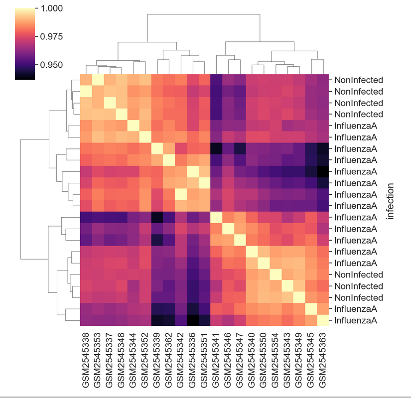
Creating a boxplot
Visualize log mean gene expression by sample and some other variable
of choice in rnaseq_df. Take some time to try to get this
plot close to publication ready for either a poster, presentation, or
paper.
You may need want to rotate the x labels of the plot, which can be
done with plt.xticks(rotation = degrees) where
degrees is the number of degrees you wish to rotate by.
Check out some of the details of sns.set_context() here.
Seaborn has useful size default for different figure types.
Your plot will of course vary, but here are some examples of what we can do:
PYTHON
sns.set_context("talk")
# Things like this will depend on your screen resolution and size
#plt.rcParams['figure.figsize'] = [8, 6]
#plt.rcParams['figure.dpi'] = 300
#sns.set(font_scale=1.25)
sns.set_palette(sns.color_palette("rocket_r", n_colors=3))
sns.boxplot(rnaseq_df,
x = "sample",
y = "log_exp",
hue = "time",
dodge=False)
plt.xticks(rotation=45, ha='right');
plt.ylabel("Log Expression")
plt.xlabel("")
# See this thread for more discussion of legend positions: https://stackoverflow.com/a/43439132
plt.legend(title='Days Post Infection', loc=(1.04, 0.5), labels=['0 days','4 days','8 days'])
PYTHON
sns.set_palette(["#A51C30","#8996A0"])
sns.violinplot(rnaseq_df,
x = "sample",
y = "log_exp",
hue = "infection",
dodge=False)
plt.xticks(rotation=45, ha='right');
plt.legend(loc = 'lower right')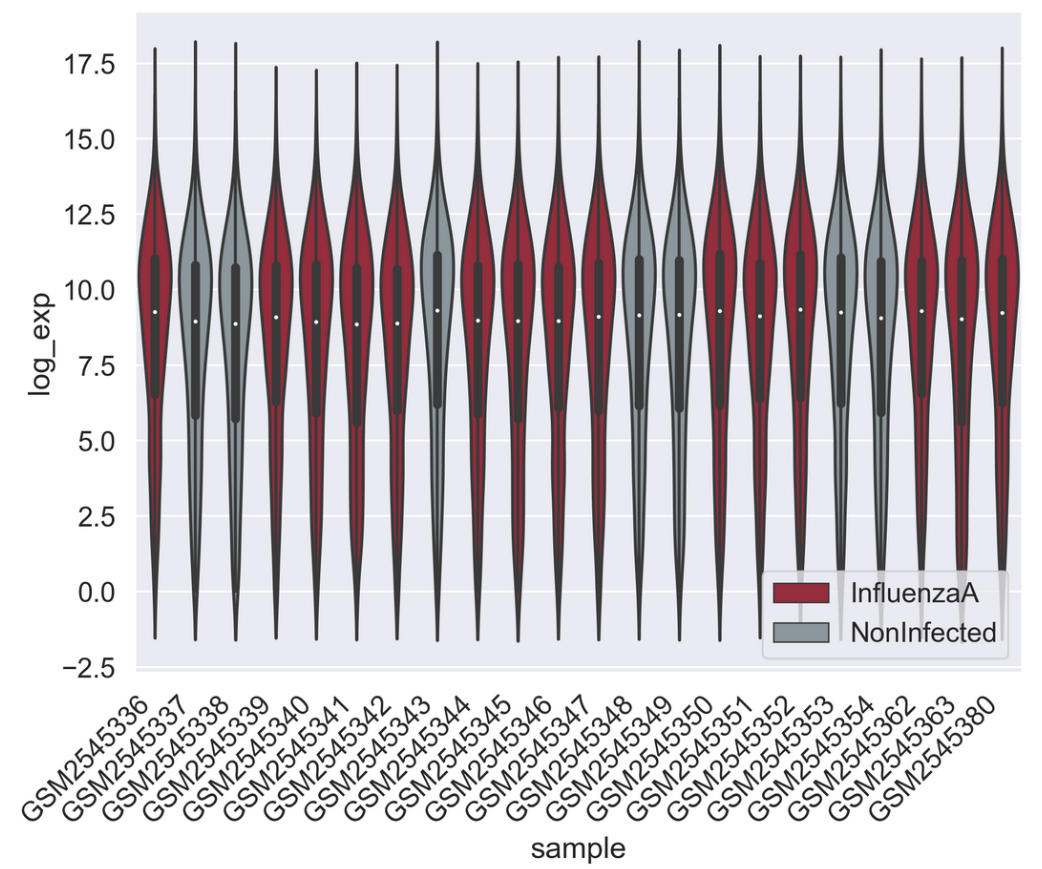
PYTHON
sns.set_context("talk")
pal = sns.color_palette("blend:#A51C30,#FFDB6D", 24)
g = sns.catplot(rnaseq_df,
kind = "box",
x = "sample",
y = "log_exp",
col = "sex",
dodge=False,
hue = "sample",
palette = pal,
sharex = False)
for axes in g.axes.flat:
_ = axes.set_xticklabels(axes.get_xticklabels(), rotation=45, ha='right')
g.set_axis_labels("", "Log Expression")
plt.subplots_adjust(wspace=0.1)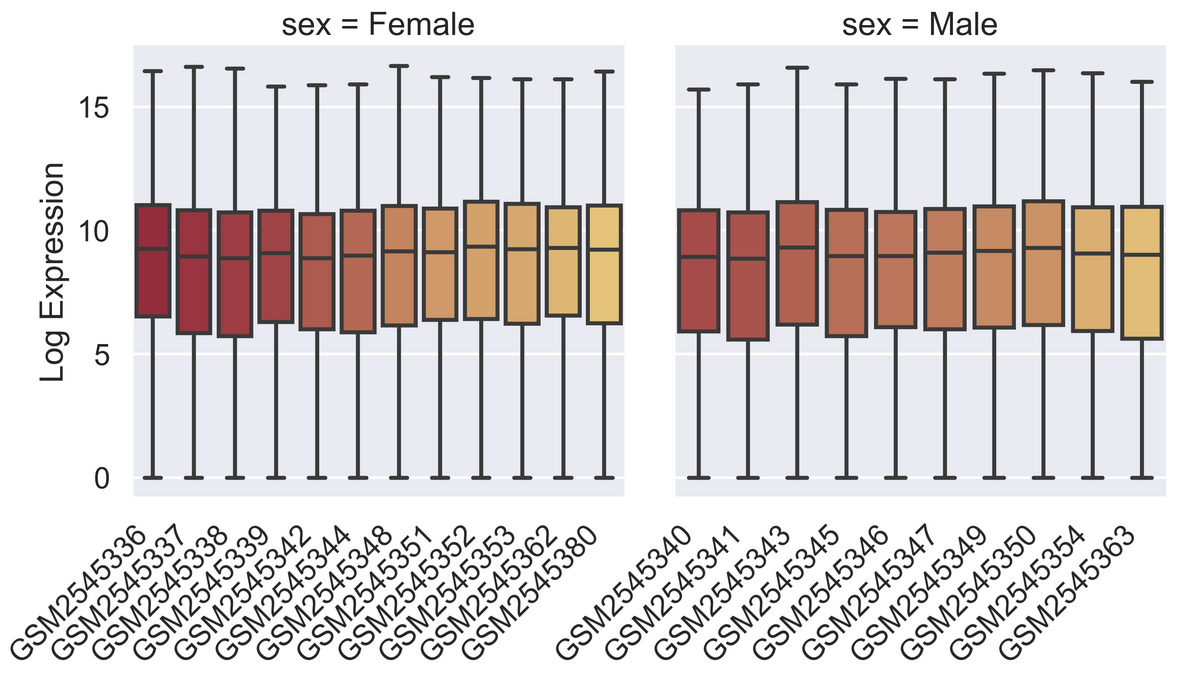
Saving your plot to a file
If you are satisfied with the plot you see you may want to save it to a file, perhaps to include it in a publication. There is a function in the matplotlib.pyplot module that accomplishes this: savefig. Calling this function, e.g. with
will save the current figure to the file my_figure.png.
The file format will automatically be deduced from the file name
extension (other formats are pdf, ps, eps and svg).
Note that functions in plt refer to a global figure
variable and after a figure has been displayed to the screen (e.g. with
plt.show) matplotlib will make this variable refer to a new
empty figure. Therefore, make sure you call plt.savefig
before the plot is displayed to the screen, otherwise you may find a
file with an empty plot.
When using dataframes, data is often generated and plotted to screen
in one line. In addition to using plt.savefig, we can save
a reference to the current figure in a local variable (with
plt.gcf) and call the savefig class method
from that variable to save the figure to file.
This supports most common image formats such as png,
svg, pdf, etc.
Making your plots accessible
Whenever you are generating plots to go into a paper or a
presentation, there are a few things you can do to make sure that
everyone can understand your plots. * Always make sure your text is
large enough to read. Use the fontsize parameter in
xlabel, ylabel, title, and
legend, and tick_params
with labelsize to increase the text size of the numbers
on your axes. * Similarly, you should make your graph elements easy to
see. Use s to increase the size of your scatterplot markers
and linewidth to increase the sizes of your plot lines. *
Using color (and nothing else) to distinguish between different plot
elements will make your plots unreadable to anyone who is colorblind, or
who happens to have a black-and-white office printer. For lines, the
linestyle parameter lets you use different types of lines.
For scatterplots, marker lets you change the shape of your
points. If you’re unsure about your colors, you can use Coblis
or Color Oracle to simulate what
your plots would look like to those with colorblindness.
Content from Perform machine learning with Scikit-learn
Last updated on 2023-04-22 | Edit this page
Overview
Questions
- What is Scikit-learn
- How is Scikit-learn used for a typical machine learning workflow?
Objectives
- Explore the
sklearnlibrary. - Walk through a typical machine learning workflow in Scikit-learn.
- Examine machine learning evaluation plots.
Key Points
- Scikit-learn is a popular package for machine learning in Python.
- Scikit-learn has a variety of useful functionality for creating predictive models.
- A machine learning workflow involves preprocessing, model selection, training, and evaluation.
Scikit-learn is a popular package for machine learning in Python.
Scikit-learn (also
called sklearn) is a popular machine learning package in
Python. It has a wide variety of functionality which aid in creating,
training, and evaluating machine learning models.
Some of its functionality includes:
- Classification: predicting a category such as active/inactive or what animal a picture is of.
- Regression: predicting a quantity such as temperature, survival
time, or age.
- Clustering: determining groupings such as trying to create groups based on the structure of the data, such as disease subtypes or celltypes.
- Dimentionality reduction: projecting data from a high-dimensional to a low-dimensional space for visualization and exploration. PCA, UMAP, and TSNE are all dimensionality reduction methods.
- Model selection: choosing which model to use. This module includes methods for splitting data for training, evaluation metrics, hyperparameter optimization, and more.
- Preprocessing: cleaning and transforming data for machine learning. This includes imputing missing data, normalization, denoising, and extracting features (for instance, creating a “season” feature from dates, or creating a “brightness” feature from an image).
Let’s import the modules and other packages we need.
Data description
The data we will be using for this lesson comes from Lee et al, 2018. In order to achieve replicative immortality, human cancer cells need to activate a telomere maintenance mechanism (TMM). Cancer cells typically use either the enzyme telomerase, or the Alternative Lengthening of Telomeres (ALT) pathway. The machine learning task we will be exporing is to create a model which can use a cancer cell’s telomere repeat composition to predict whether or not a tumor cell is using the ALT pathway.
More formally, we are predicting a binary variable for each sample, whether the TMM is using the ALT pathway (positive) or not (negative). In machine learning we refer to this as the target variable or class of the data. We have set of columns in the dataset which indicate the six-mer composition of the sample’s telomeres by percent.
PYTHON
# Load data
data = pd.read_csv("https://raw.githubusercontent.com/HMS-Data-Club/python-environments/main/data/telomere_ALT/telomere.csv", sep='\t')
num_row = data.shape[0] # number of samples in the dataset
num_col = data.shape[1] # number of features in the dataset (plus the label column)
print(data)OUTPUT
TTAGGG ATAGGG CTAGGG GTAGGG TAAGGG TCAGGG TGAGGG TTCGGG TTGGGG \
0 94.846 0.019 0.430 0.422 0.216 0.544 1.762 0.535 0.338
1 94.951 0.011 0.241 0.491 0.223 0.317 1.351 0.818 0.702
2 94.889 0.043 0.439 0.478 0.355 0.316 1.151 0.625 0.313
3 94.202 0.017 0.252 0.509 0.396 0.548 1.877 0.856 0.440
4 96.368 0.011 0.078 0.131 0.015 0.306 1.525 1.165 0.126
.. ... ... ... ... ... ... ... ... ...
156 98.608 0.001 0.100 0.219 0.000 0.196 0.421 0.101 0.229
157 98.176 0.000 0.145 0.304 0.088 0.158 0.446 0.181 0.292
158 99.393 0.000 0.017 0.155 0.000 0.030 0.190 0.065 0.073
159 98.742 0.003 0.077 0.169 0.002 0.091 0.304 0.211 0.206
160 98.738 0.009 0.138 0.113 0.000 0.371 0.186 0.080 0.163
TTTGGG ... TTACGG TTATGG TTAGAG TTAGCG TTAGTG TTAGGA TTAGGC \
0 0.068 ... 0.028 0.118 0.153 0.000 0.049 0.060 0.033
1 0.090 ... 0.024 0.125 0.080 0.024 0.035 0.155 0.030
2 0.079 ... 0.041 0.253 0.195 0.032 0.043 0.161 0.047
3 0.097 ... 0.053 0.110 0.125 0.000 0.043 0.069 0.029
4 0.000 ... 0.014 0.099 0.022 0.000 0.019 0.026 0.009
.. ... ... ... ... ... ... ... ... ...
156 0.000 ... 0.019 0.020 0.016 0.000 0.004 0.025 0.011
157 0.023 ... 0.012 0.013 0.043 0.000 0.005 0.009 0.015
158 0.000 ... 0.008 0.014 0.009 0.000 0.003 0.012 0.013
159 0.000 ... 0.011 0.053 0.047 0.000 0.004 0.019 0.014
160 0.000 ... 0.015 0.049 0.023 0.000 0.021 0.037 0.021
TTAGGT rel_TL TMM
0 0.089 -0.89 -
1 0.093 -0.39 -
2 0.185 -1.66 -
3 0.110 -1.73 -
4 0.014 0.21 -
.. ... ... ...
156 0.001 2.00 +
157 0.013 0.98 +
158 0.003 1.29 +
159 0.007 1.24 +
160 0.009 1.71 +
[161 rows x 21 columns]Machine learning workflows involves preprocessing, model selection, training, and evaluation.
Before we can use a model to predict ALT pathway activity, however, we have to do three steps: 1. Preprocessing: Gather data and get it ready for use in the machine learning model. 2. Learning/Training: Choose a machine learning model and train it on the data. 3. Evaluation: Measure how well the model performed. Can we trust the predictions of the trained model?
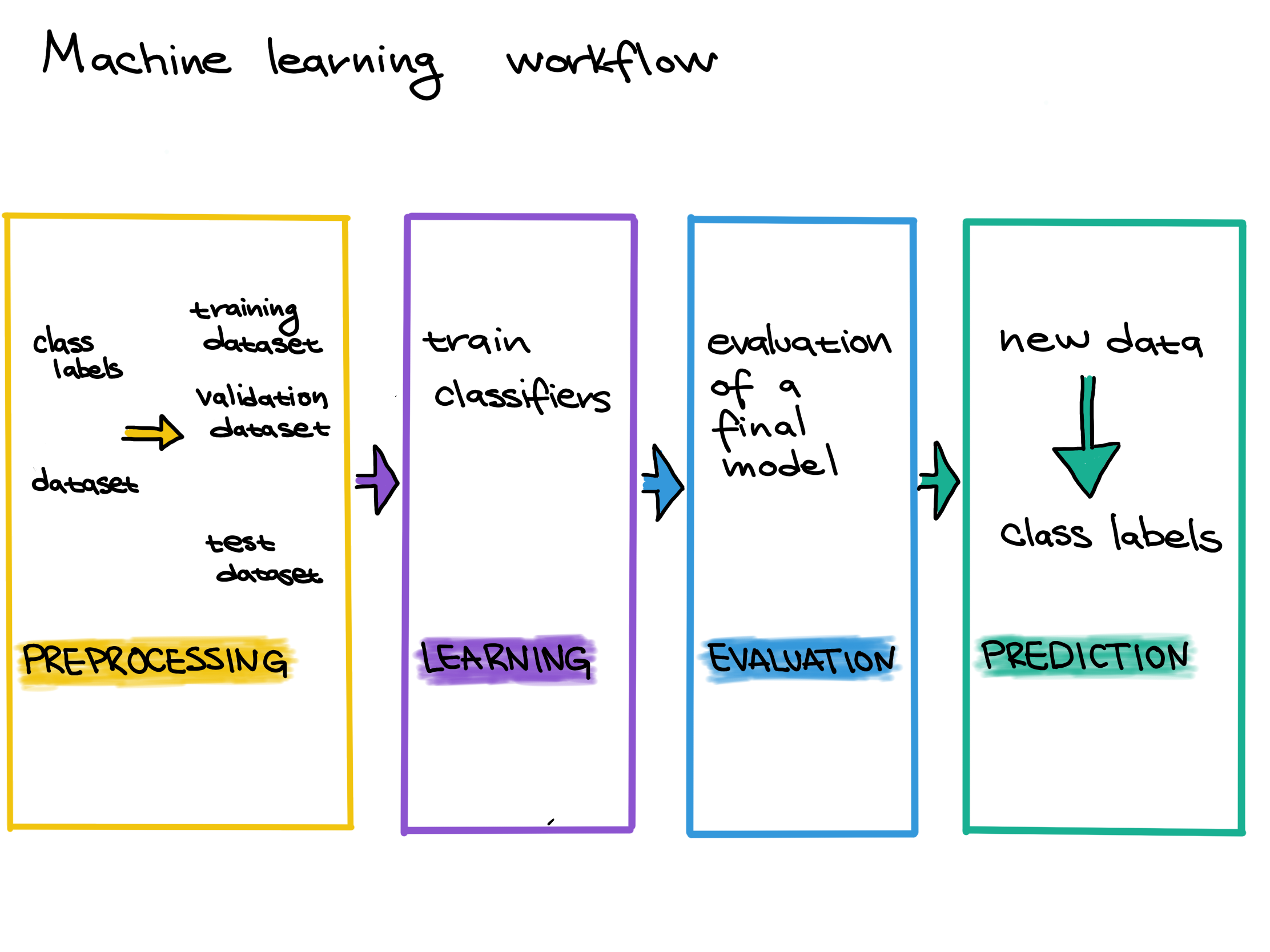
In this case, our data is already preprocessed. In order to perform training, we need to split our data into a training set and a testing set.
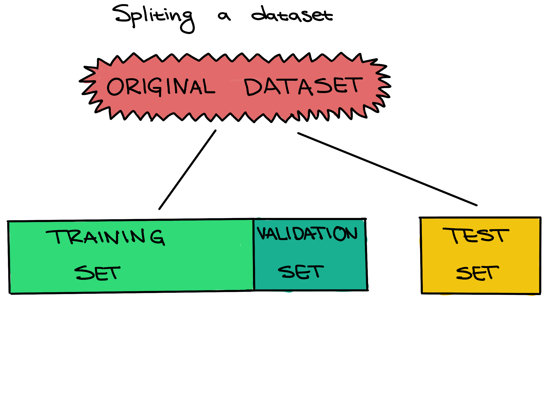 .
.
Scikit-learn has useful built-in functions for splitting data inside
of its model_selection module. Here, we use
train_test_split. The convention in Scikit-learn (as well
as more generally in machine learning) is to call our feactures
X and our target variable y.
PYTHON
X = data.iloc[:, 0: num_col-1] # feature columns
y = data['TMM'] # label column
X_train, X_test, y_train, y_test = \
model_selection.train_test_split(X, y,
test_size=0.2, # reserve 20 percent data for testing
stratify=y, # stratified sampling
random_state=0) # random seedSetting a test set aside from the training and validation sets from the beginning, and only using it once for a final evaluation, is very important to be able to properly evaluate how well a machine learning algorithm learned. If this data leakage occurs it contaminates the evaluation, making the evaluation not accurately reflect how well the model actually performs. Letting the machine learning method learn from the test set can be seen as giving a student the answers to an exam; once a student sees any exam answers, their exam score will no longer reflect their true understanding of the material.
In other words, improper data splitting and data leakage means that we will not know if our model works or not.
Now that we have our data split up, we can select and train our model, in machine learning tasks like this also called our classifier. We want to further split our training data into a traiing set and validation set so that we can freely explore different models before making our final choice.
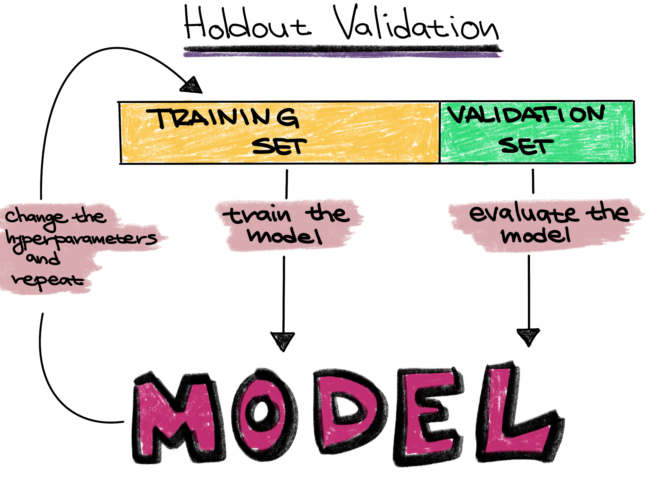
However, in this case we are simply going to go with a random forest classifier. Random forests are a fast classifier which tends to perform well, and is often reccomended as a first classifier to try.
Definitions
Training set - The training set is a part of the original dataset that trains or fits the model. This is the data that the model uses to learn patterns and set the model parameters.
Validation set - Part of the training set is used to validate that the fitted model works on new data. This is not the final evaluation of the model. This step is used to change hyperparameters and then train the model again.
Test set - The test set checks how well we expect the model to work on new data in the future. The test set is used in the final phase of the workflow, and it evaluates the final model. It can only be used one time, and the model cannot be adjusted after using it.
Parameters - These are the aspects of a machine learning model that are learned from the training data. The parameters define the prediction rules of the trained model.
Hyperparameters - These are the user-specified settings of a machine learning model. Each machine learning method has different hyperparameters, and they control various trade-offs which change how the model learns. Hyperparameters control parts of a machine learning method such as how much emphasis the method should place on being perfectly correct versus becoming overly complex, how fast the method should learn, the type of mathematical model the method should use for learning, and more.
Model Creation
PYTHON
rf = ensemble.RandomForestClassifier(
n_estimators = 10, # 10 random trees in the forest
criterion = 'entropy', # use entropy as the measure of uncertainty
max_depth = 3, # maximum depth of each tree is 3
min_samples_split = 5, # generate a split only when there are at least 5 samples at current node
class_weight = 'balanced', # class weight is inversely proportional to class frequencies
random_state = 0)Each model in Scikit-learn has a wide variety of possible hyperparameters to choose from. These can be thought of as the settings, or knobs and dials, of the model.
Once we’ve created the model, in Scikit-learn we train it using the
fit method on the training data. We can then look at its
score on the testing data using the score method.
Training
PYTHON
# Refit the classifier using the full training set
rf = rf.fit(X_train, y_train)
# Compute classifier's accuracy on the test set
test_accuracy = rf.score(X_test, y_test)
print(f'Test accuracy: {test_accuracy: 0.3f}')OUTPUT
Test accuracy: 0.848Evaluation
This means that we predicted the TMM correctly in about 85% of our
test samples. As oppsed to the score, we can also directly get each of
the model’s predictions. We can either use predict to get a
single prediction or predict_proba to get a probablistic
confidence score.
PYTHON
# Predict labels for the test set
y = rf.predict(X_test) # Solid prediction
y_prob = rf.predict_proba(X_test) # Soft prediction
print(y)
print(y_prob)OUTPUT
['+' '+' '+' '-' '-' '+' '+' '-' '-' '-' '+' '-' '+' '-' '-' '+' '-' '-'
'-' '-' '+' '-' '-' '+' '-' '-' '-' '-' '-' '-' '+' '+' '+']
[[0.81355661 0.18644339]
[0.85375 0.14625 ]
[0.72272654 0.27727346]
[0.03321429 0.96678571]
[0.04132653 0.95867347]
[0.98434442 0.01565558]
[0.99230769 0.00769231]
[0.09321429 0.90678571]
[0.0225 0.9775 ]
[0.08788497 0.91211503]
[0.99238014 0.00761986]
[0. 1. ]
[0.87857143 0.12142857]
[0.0225 0.9775 ]
[0.1 0.9 ]
[0.52973416 0.47026584]
[0.17481069 0.82518931]
[0.29859926 0.70140074]
[0.43977573 0.56022427]
[0. 1. ]
[0.80117647 0.19882353]
[0.03061224 0.96938776]
[0.22071729 0.77928271]
[0.72899028 0.27100972]
[0.0975 0.9025 ]
[0. 1. ]
[0.03061224 0.96938776]
[0. 1. ]
[0.45651511 0.54348489]
[0.1 0.9 ]
[0.81355661 0.18644339]
[0.85375 0.14625 ]
[0.88516484 0.11483516]]Instead of simple metrics such as accuracy which can be misleading, we can also look at and plot more complex metrics such as the receiver operating characteristic (ROC) curve or the precision recall (PR) curve.
PYTHON
# Compute the ROC and PR curves for the test set
fpr, tpr, _ = metrics.roc_curve(y_test, y_prob[:, 0], pos_label='+')
precision_plus, recall_plus, _ = metrics.precision_recall_curve(y_test, y_prob[:, 0], pos_label='+')
precision_minus, recall_minus, _ = metrics.precision_recall_curve(y_test, y_prob[:, 1], pos_label='-')
# Compute the AUROC and AUPRCs for the test set
auroc = metrics.auc(fpr, tpr)
auprc_plus = metrics.auc(recall_plus, precision_plus)
auprc_minus = metrics.auc(recall_minus, precision_minus)
# Plot the ROC curve for the test set
plt.plot(fpr, tpr, label='test (area = %.3f)' % auroc)
plt.plot([0,1], [0,1], linestyle='--', color=(0.6, 0.6, 0.6))
plt.plot([0,0,1], [0,1,1], linestyle='--', color=(0.6, 0.6, 0.6))
plt.xlim([-0.05, 1.05])
plt.ylim([-0.05, 1.05])
plt.xlabel('FPR')
plt.ylabel('TPR')
plt.legend(loc='lower right')
plt.title('ROC curve')
plt.show()
# Plot the PR curve for the test set
plt.plot(recall_plus, precision_plus, label='positive class (area = %.3f)' % auprc_plus)
plt.plot(recall_minus, precision_minus, label='negative class (area = %.3f)' % auprc_minus)
plt.plot([0,1,1], [1,1,0], linestyle='--', color=(0.6, 0.6, 0.6))
plt.xlim([-0.05, 1.05])
plt.ylim([-0.05, 1.05])
plt.xlabel('recall')
plt.ylabel('precision')
plt.legend(loc='lower left')
plt.title('Precision-recall curve')
plt.show()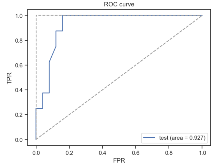
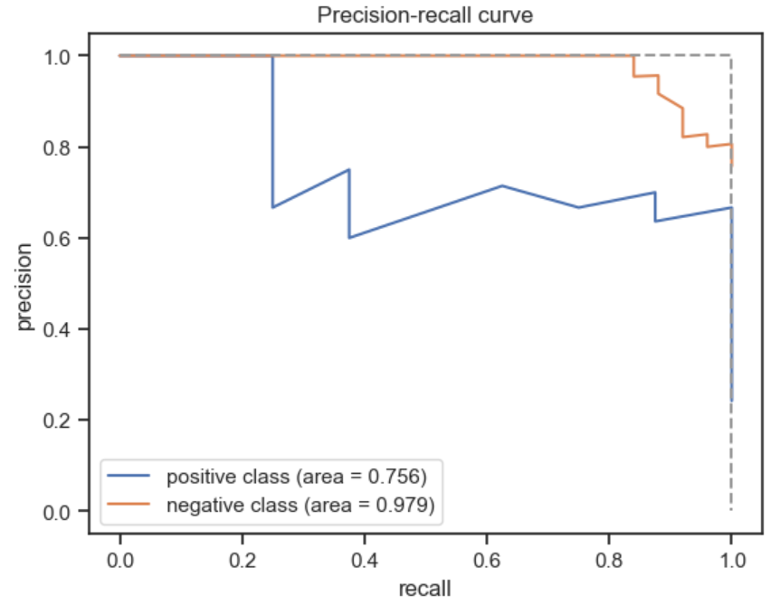
Finally, we can also look at the confusion matrix, another useful summary of model performance.
PYTHON
# Compute the confusion matrix for the test set
cm = metrics.confusion_matrix(y_test, y)
# Plot the confusion matrix for the test set
plt.matshow(cm, interpolation='nearest', cmap=plt.cm.Blues, alpha=0.5)
plt.xticks(np.arange(2), ('+', '-'))
plt.yticks(np.arange(2), ('+', '-'))
for i in range(2):
for j in range(2):
plt.text(j, i, cm[i, j], ha='center', va='center')
plt.xlabel('Predicted label')
plt.ylabel('True label')
plt.show()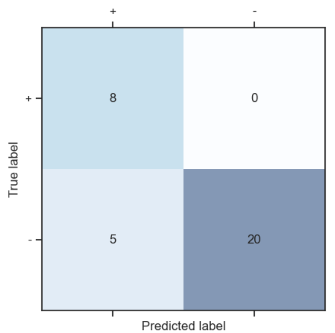
Resources for learning more
The Google machine learning glossary and ML4Bio guides define common machine learning terms.
The scikit-learn tutorials provide a Python-based introduction to machine learning. There is also a third-party scikit-learn tutorial and a Carpentries lesson.
The book Python Machine Learning has machine learning example code.
The Elements of AI course presents general introductory materials to machine learning and related topics.
Galaxy ML provides access to classification and regression workflows through the Galaxy interface.
You can find additional resources at these links for beginners and intermediate users.
Content from ID mapping using mygene
Last updated on 2023-04-27 | Edit this page
Overview
Questions
- How can I get gene annotations in Python?
Objectives
- Explore the
mygenelibrary. - Access and merge gene annotations using
mygene.
Key Points
-
mygeneis Python module which allows access to a gene annotation database. - You can query
mygenewith multiple identifiers usingquerymany.
Installing mygene from bioconda
ID mapping is a very common, often not fun, task for every bioinformatician. Different datasets and tools often use different sets of biological identifiers. Our goal is to take some list of gene symbols other gene identifiers and convert them to some other set of identifiers to facilitate some analysis.
mygene is a convenient Python module to access MyGene.info gene query web services.
Mygene is a part of a family of biothings API services which also has modules for chemical, diseases, genetic variances, and taxonomy. All of these modules use a simlar Python interface.
Mygene can be installed using conda, but we it exists on a separate
set of biomedical packages called bioconda. We access this using
the -c flag which tells conda the channel we wish
to search.
Once installed, we can import mygene and create a
MyGeneInfo object, which is used for accessing and
downloading genetic annotations.
Mapping gene symbols
Suppose xli is a list of gene symbols we want to convert to entrez gene ids:
PYTHON
xli = ['DDX26B',
'CCDC83',
'MAST3',
'FLOT1',
'RPL11',
'ZDHHC20',
'LUC7L3',
'SNORD49A',
'CTSH',
'ACOT8']We can then use the querymany method to get entrez
gene ids for this list, telling it your input is “symbol” with the
scopes argument, and you want “entrezgene” (Entrez gene
ids) back with the fields argument.
OUTPUT
querying 1-10...done.
Finished.
1 input query terms found no hit:
['DDX26B']
Pass "returnall=True" to return complete lists of duplicate or missing query terms.
[{'query': 'DDX26B', 'notfound': True}, {'query': 'CCDC83', '_id': '220047', '_score': 18.026102, 'entrezgene': '220047'}, {'query': 'MAST3', '_id': '23031', '_score': 18.120222, 'entrezgene': '23031'}, {'query': 'FLOT1', '_id': '10211', '_score': 18.43404, 'entrezgene': '10211'}, {'query': 'RPL11', '_id': '6135', '_score': 16.711576, 'entrezgene': '6135'}, {'query': 'ZDHHC20', '_id': '253832', '_score': 18.165747, 'entrezgene': '253832'}, {'query': 'LUC7L3', '_id': '51747', '_score': 17.696375, 'entrezgene': '51747'}, {'query': 'SNORD49A', '_id': '26800', '_score': 22.741982, 'entrezgene': '26800'}, {'query': 'CTSH', '_id': '1512', '_score': 17.737492, 'entrezgene': '1512'}, {'query': 'ACOT8', '_id': '10005', '_score': 17.711779, 'entrezgene': '10005'}]The mapping result is returned as a list of dictionaries. Each dictionary contains the fields we asked to return, in this case, “entrezgene” field. Each dictionary also returns the matching query term, “query”, and an internal id, “**_id“, which is the same as”entrezgene**” most of time (will be an ensembl gene id if a gene is available from Ensembl only). Mygene could not find a mapping for one of the genes.
We could also get Ensembl gene ids. This time, we will use the
as.dataframe argument to get the result back as a pandas
dataframe.
PYTHON
ensembl_res = mg.querymany(xli, scopes='symbol', fields='ensembl.gene', species='human', as_dataframe=True)
print(ensembl_res)OUTPUT
querying 1-10...done.
Finished.
1 input query terms found no hit:
['DDX26B']
Pass "returnall=True" to return complete lists of duplicate or missing query terms.
notfound _id _score ensembl.gene \
query
DDX26B True NaN NaN NaN
CCDC83 NaN 220047 18.026253 ENSG00000150676
MAST3 NaN 23031 18.120222 ENSG00000099308
FLOT1 NaN 10211 18.416580 NaN
RPL11 NaN 6135 16.711576 ENSG00000142676
ZDHHC20 NaN 253832 18.165747 ENSG00000180776
LUC7L3 NaN 51747 17.701532 ENSG00000108848
SNORD49A NaN 26800 22.728123 ENSG00000277370
CTSH NaN 1512 17.725145 ENSG00000103811
ACOT8 NaN 10005 17.717607 ENSG00000101473
ensembl
query
DDX26B NaN
CCDC83 NaN
MAST3 NaN
FLOT1 [{'gene': 'ENSG00000206480'}, {'gene': 'ENSG00...
RPL11 NaN
ZDHHC20 NaN
LUC7L3 NaN
SNORD49A NaN
CTSH NaN
ACOT8 NaN Mixed symbols and multiple fields
The above id list contains multiple types of identifiers. Let’s try taking this list and trying to get back both Entrez gene ids and uniprot ids. Parameters scopes, fields, species are all flexible enough to support multiple values, either a list or a comma-separated string.
PYTHON
query_res = mg.querymany(xli, scopes='symbol,reporter,accession,ensembl.gene', fields='entrezgene,uniprot', species='human', as_dataframe=True)
print(query_res)OUTPUT
querying 1-6...done.
Finished.
1 input query terms found dup hits:
[('1007_s_at', 2)]
Pass "returnall=True" to return complete lists of duplicate or missing query terms.
_id _score entrezgene uniprot.Swiss-Prot \
query
ENSG00000150676 220047 24.495731 220047 Q8IWF9
MAST3 23031 18.115461 23031 O60307
FLOT1 10211 18.416580 10211 O75955
RPL11 6135 16.715294 6135 P62913
1007_s_at 100616237 18.266214 100616237 NaN
1007_s_at 780 18.266214 780 Q08345
AK125780 118142757 21.342941 118142757 P43080
uniprot.TrEMBL
query
ENSG00000150676 H0YDV3
MAST3 [V9GYV0, A0A8V8TLL8, A0A8I5KST9, A0A8V8TMW0, A...
FLOT1 [A2AB11, Q5ST80, A2AB13, A2AB10, A2ABJ5, A2AB1...
RPL11 [Q5VVC8, Q5VVD0, A0A2R8Y447]
1007_s_at NaN
1007_s_at [A0A024RCJ0, A0A024RCL1, A0A0A0MSX3, A0A024RCQ...
AK125780 [A0A7I2V6E2, B2R9P6] Finally, we can take a look at all of the information mygene has to
offer by setting fields to “all”.
PYTHON
query_res = mg.querymany(xli, scopes='symbol,reporter,accession,ensembl.gene', fields='all', species='human', as_dataframe=True)
print(list(query_res.columns))OUTPUT
querying 1-6...done.
Finished.
1 input query terms found dup hits:
[('1007_s_at', 2)]
Pass "returnall=True" to return complete lists of duplicate or missing query terms.
['AllianceGenome', 'HGNC', '_id', '_score', 'alias', 'entrezgene', 'exons', 'exons_hg19', 'generif', 'ipi', 'map_location', 'name', 'other_names', 'pharmgkb', 'symbol', 'taxid', 'type_of_gene', 'unigene', 'accession.genomic', 'accession.protein', 'accession.rna', 'accession.translation', 'ensembl.gene', 'ensembl.protein', 'ensembl.transcript', 'ensembl.translation', 'ensembl.type_of_gene', 'exac._license', 'exac.all.exp_lof', 'exac.all.exp_mis', 'exac.all.exp_syn', 'exac.all.lof_z', 'exac.all.mis_z', 'exac.all.mu_lof', 'exac.all.mu_mis', 'exac.all.mu_syn', 'exac.all.n_lof', 'exac.all.n_mis', 'exac.all.n_syn', 'exac.all.p_li', 'exac.all.p_null', 'exac.all.p_rec', 'exac.all.syn_z', 'exac.bp', 'exac.cds_end', 'exac.cds_start', 'exac.n_exons', 'exac.nonpsych.exp_lof', 'exac.nonpsych.exp_mis', 'exac.nonpsych.exp_syn', 'exac.nonpsych.lof_z', 'exac.nonpsych.mis_z', 'exac.nonpsych.mu_lof', 'exac.nonpsych.mu_mis', 'exac.nonpsych.mu_syn', 'exac.nonpsych.n_lof', 'exac.nonpsych.n_mis', 'exac.nonpsych.n_syn', 'exac.nonpsych.p_li', 'exac.nonpsych.p_null', 'exac.nonpsych.p_rec', 'exac.nonpsych.syn_z', 'exac.nontcga.exp_lof', 'exac.nontcga.exp_mis', 'exac.nontcga.exp_syn', 'exac.nontcga.lof_z', 'exac.nontcga.mis_z', 'exac.nontcga.mu_lof', 'exac.nontcga.mu_mis', 'exac.nontcga.mu_syn', 'exac.nontcga.n_lof', 'exac.nontcga.n_mis', 'exac.nontcga.n_syn', 'exac.nontcga.p_li', 'exac.nontcga.p_null', 'exac.nontcga.p_rec', 'exac.nontcga.syn_z', 'exac.transcript', 'genomic_pos.chr', 'genomic_pos.end', 'genomic_pos.ensemblgene', 'genomic_pos.start', 'genomic_pos.strand', 'genomic_pos_hg19.chr', 'genomic_pos_hg19.end', 'genomic_pos_hg19.start', 'genomic_pos_hg19.strand', 'go.MF.category', 'go.MF.evidence', 'go.MF.id', 'go.MF.pubmed', 'go.MF.qualifier', 'go.MF.term', 'homologene.genes', 'homologene.id', 'interpro.desc', 'interpro.id', 'interpro.short_desc', 'pantherdb.HGNC', 'pantherdb._license', 'pantherdb.ortholog', 'pantherdb.uniprot_kb', 'pharos.target_id', 'reagent.GNF_Qia_hs-genome_v1_siRNA', 'reagent.GNF_hs-ORFeome1_1_reads.id', 'reagent.GNF_hs-ORFeome1_1_reads.relationship', 'reagent.GNF_mm+hs-MGC.id', 'reagent.GNF_mm+hs-MGC.relationship', 'reagent.GNF_mm+hs_RetroCDNA.id', 'reagent.GNF_mm+hs_RetroCDNA.relationship', 'reagent.NOVART_hs-genome_siRNA', 'refseq.genomic', 'refseq.protein', 'refseq.rna', 'refseq.translation', 'reporter.GNF1H', 'reporter.HG-U133_Plus_2', 'reporter.HTA-2_0', 'reporter.HuEx-1_0', 'reporter.HuGene-1_1', 'reporter.HuGene-2_1', 'umls.cui', 'uniprot.Swiss-Prot', 'uniprot.TrEMBL', 'MIM', 'ec', 'interpro', 'pdb', 'pfam', 'prosite', 'summary', 'go.BP', 'go.CC.evidence', 'go.CC.gocategory', 'go.CC.id', 'go.CC.qualifier', 'go.CC.term', 'go.MF', 'reagent.GNF_hs-Origene.id', 'reagent.GNF_hs-Origene.relationship', 'reagent.GNF_hs-druggable_lenti-shRNA', 'reagent.GNF_hs-druggable_plasmid-shRNA', 'reagent.GNF_hs-druggable_siRNA', 'reagent.GNF_hs-pkinase_IDT-siRNA', 'reagent.Invitrogen_IVTHSSIPKv2', 'reagent.NIBRI_hs-Secretome_pDEST.id', 'reagent.NIBRI_hs-Secretome_pDEST.relationship', 'reporter.HG-U95Av2', 'ensembl', 'genomic_pos', 'genomic_pos_hg19', 'go.CC', 'pathway.kegg.id', 'pathway.kegg.name', 'pathway.netpath.id', 'pathway.netpath.name', 'pathway.reactome', 'pathway.wikipathways', 'reagent.GNF_hs-Origene', 'wikipedia.url_stub', 'pir', 'pathway.kegg', 'pathway.pid', 'pathway.wikipathways.id', 'pathway.wikipathways.name', 'miRBase', 'retired', 'reagent.GNF_mm+hs-MGC'You can find a neater version of all available fields here.
Challenge
Load in the rnaseq dataset as a pandas dataframe. Add columns to the dataframe with entrez gene ids and at least one other field from mygene.
Other bioinformatics resources
Biopython is a library with a wide variety of bioinformatics applications. You can find its tutorial/cookbook here
This lesson was adapted from the official mygene python tutorial