Reshaping Data
Last updated on 2023-04-27 | Edit this page
Overview
Questions
- How can change the shape of my data?
- What is the difference between long and wide data?
Objectives
- Extract substrings of interest.
- Format dynamic strings using f-strings.
- Explore Python’s built-in string functions
Key Points
- Strings can be indexed and sliced.
- Strings cannot be directly altered.
- You can build complex strings based on other variables using f-strings and format.
- Python has a variety of useful built-in string functions.
Wide data and long data
We’ve so far seen our gene expression dataset in two distinct formats which we used for different purposes.
Our original dataset contains a single count value per row, and has all metadata included:
PYTHON
import pandas as pd

url = "https://raw.githubusercontent.com/ccb-hms/workbench-python-workshop/main/episodes/data/rnaseq_reduced.csv"
rnaseq_df = pd.read_csv(url)
print(rnaseq_df)
OUTPUT
         gene      sample  expression  time
0         Asl  GSM2545336        1170     8
1        Apod  GSM2545336       36194     8
2     Cyp2d22  GSM2545336        4060     8
3        Klk6  GSM2545336         287     8
4       Fcrls  GSM2545336          85     8
...       ...         ...         ...   ...
7365    Mgst3  GSM2545340        1563     4
7366   Lrrc52  GSM2545340           2     4
7367     Rxrg  GSM2545340          26     4
7368    Lmx1a  GSM2545340          81     4
7369     Pbx1  GSM2545340        3805     4

[7370 rows x 4 columns]
Data in this format is referred to as long data.
We also looked at a version of the same data which only contained expression data, where each sample was a column:
PYTHON
url = "https://raw.githubusercontent.com/ccb-hms/workbench-python-workshop/main/episodes/data/expression_matrix.csv"
expression_matrix = pd.read_csv(url, index_col=0)
print(expression_matrix.iloc[:10, :5])
OUTPUT
          GSM2545336  GSM2545337  GSM2545338  GSM2545339  GSM2545340
gene
AI504432        1230        1085         969        1284         966
AW046200          83         144         129         121         141
AW551984         670         265         202         682         246
Aamp            5621        4049        3797        4375        4095
Abca12             5           8           1           5           3
Abcc8           2210        1966        2181        2362        2475
Abhd14a          490         495         474         468         489
Abi2            5627        4383        4107        4062        4289
Abi3bp           807        1144        1028         935         879
Abl2            2392        2133        1891        1645        1926
Data in this format is referred to as wide data.
Each format has its pros and cons, and we often need to switch between the two. Wide data is more human readable, and allows for easy comparision across different samples, such as finding the genes with the highest average expression. However, wide data requires any sample metadata to exist as a separate dataframe. Thus it is much more difficult to examine sample metadata, such as calculating the mean expression at a particular timepoint.
In contrast, long data is considered less human readable. We have to first aggregate our data by gene if we want to do something like calculate average expression. However, we can easily group the data by whatever sample metadata we wish. We will also see in the next session that long data is the preferred format for plotting.
Wide and long data also handle missing data differently. In long
data, and values which don’t exist for a particular sample simply aren’t
rows in the dataset. Thus, our data does not have null
values, but it is harder to tell where data is missing. In wide data,
there is a matrix position for every combination of sample and gene.
Thus, any missing data is shown as a null value. This can
be more difficult to deal with, but makes missing data clear.
Convert from wide to long with melt.
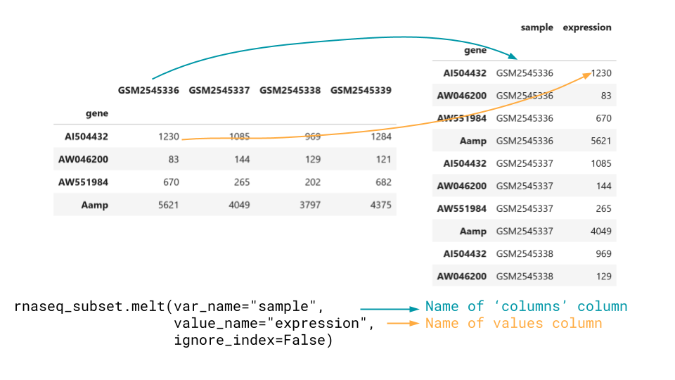
We can convert from wide data to long data using melt.
melt takes in the arguments var_name and
value_name, which are strings that name the two created
columns. We also typically want to set the ignore_index
argument to False, otherwise pandas will drop the dataframe
index.
We could also allow pandas to drop the index, if there is some other
column we want the new rows to be named by, and pass that in instead as
the id_vars argument.
PYTHON
long_data = expression_matrix.melt(var_name="sample", value_name="expression", ignore_index=False)
print(long_data)
OUTPUT
              sample  expression
gene
AI504432  GSM2545336        1230
AW046200  GSM2545336          83
AW551984  GSM2545336         670
Aamp      GSM2545336        5621
Abca12    GSM2545336           5
...              ...         ...
Zkscan3   GSM2545380        1900
Zranb1    GSM2545380        9942
Zranb3    GSM2545380         202
Zscan22   GSM2545380         527
Zw10      GSM2545380        1664

[32428 rows x 2 columns]
Convert from long to wide with pivot.
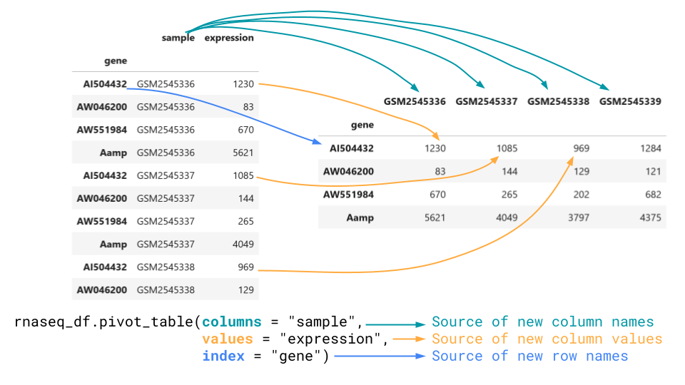
To go the other way, we want to use the pivot_table method.
This method takes in a columns the column to get new
column names from, values, what to populate the matrix
with, and index, what the row names of the wide data should
be.
PYTHON
wide_data = rnaseq_df.pivot_table(columns = "sample", values = "expression", index = "gene")
print(wide_data)
OUTPUT
sample    GSM2545336  GSM2545337  GSM2545338  GSM2545339  GSM2545340
gene
AI504432        1230        1085         969        1284         966
AW046200          83         144         129         121         141
AW551984         670         265         202         682         246
Aamp            5621        4049        3797        4375        4095
Abca12             5           8           1           5           3
...              ...         ...         ...         ...         ...
Zkscan3         1732        1840        1800        1751        2056
Zranb1          8837        5306        5106        5306        5896
Zranb3           207         179         199         208         184
Zscan22          483         535         533         462         439
Zw10            1479        1394        1279        1376        1568

[1474 rows x 5 columns]
Note that any columns in the dataframe which are not used as values are dropped.
Challenge
Create a dataframe of the rnaseq dataset where each row is a gene and each column is a timepoint instead of a sample. The values in each column should be the mean count across all samples at that timepoint.
Take a look at the aggfunc argument in pivot_table.
What is the default?