R Basics

Extended Materials

You can find the original, extended version of this chapter here.

Data Preparation

library(rio)
library(here)
library(apyramid)
library(dplyr)
linelist <- rio::import("data/case_linelists/linelist_cleaned.rds")

Functions

Functions are at the core of using R. Functions are how you perform tasks and operations. Many functions come installed with R, many more are available for download in packages (explained in the packages section), and you can even write your own custom functions!

This basics section on functions explains:

What a function is and how they work
What function arguments are
How to get help understanding a function

A quick note on syntax

In this workbook, functions are written in code-text with open parentheses, like this: filter(). As explained in the packages section, functions are downloaded within packages. In this handbook, package names are written in bold, like dplyr. Sometimes in example code you may see the function name linked explicitly to the name of its package with two colons (::) like this: dplyr::filter(). The purpose of this linkage is explained in the packages section.

Simple functions

A function is like a machine that receives inputs, does some action with those inputs, and produces an output. What the output is depends on the function.

Functions typically operate upon some object placed within the function’s parentheses. For example, the function sqrt() calculates the square root of a number:

sqrt(49)

[1] 7

The object provided to a function also can be a column in a dataset (see the Objects section for detail on all the kinds of objects). Because R can store multiple datasets, you will need to specify both the dataset and the column. One way to do this is using the $ notation to link the name of the dataset and the name of the column (dataset$column). In the example below, the function summary() is applied to the numeric column age in the dataset linelist, and the output is a summary of the column’s numeric and missing values.

# Print summary statistics of column 'age' in the dataset 'linelist'
summary(linelist$age)

   Min. 1st Qu.  Median    Mean 3rd Qu.    Max.    NA's 
   0.00    6.00   13.00   16.07   23.00   84.00      86

Note

Behind the scenes, a function represents complex additional code that has been wrapped up for the user into one easy command.

Functions with multiple arguments

Functions often ask for several inputs, called arguments, located within the parentheses of the function, usually separated by commas.

Some arguments are required for the function to work correctly, others are optional
Optional arguments have default settings
Arguments can take character, numeric, logical (TRUE/FALSE), and other inputs

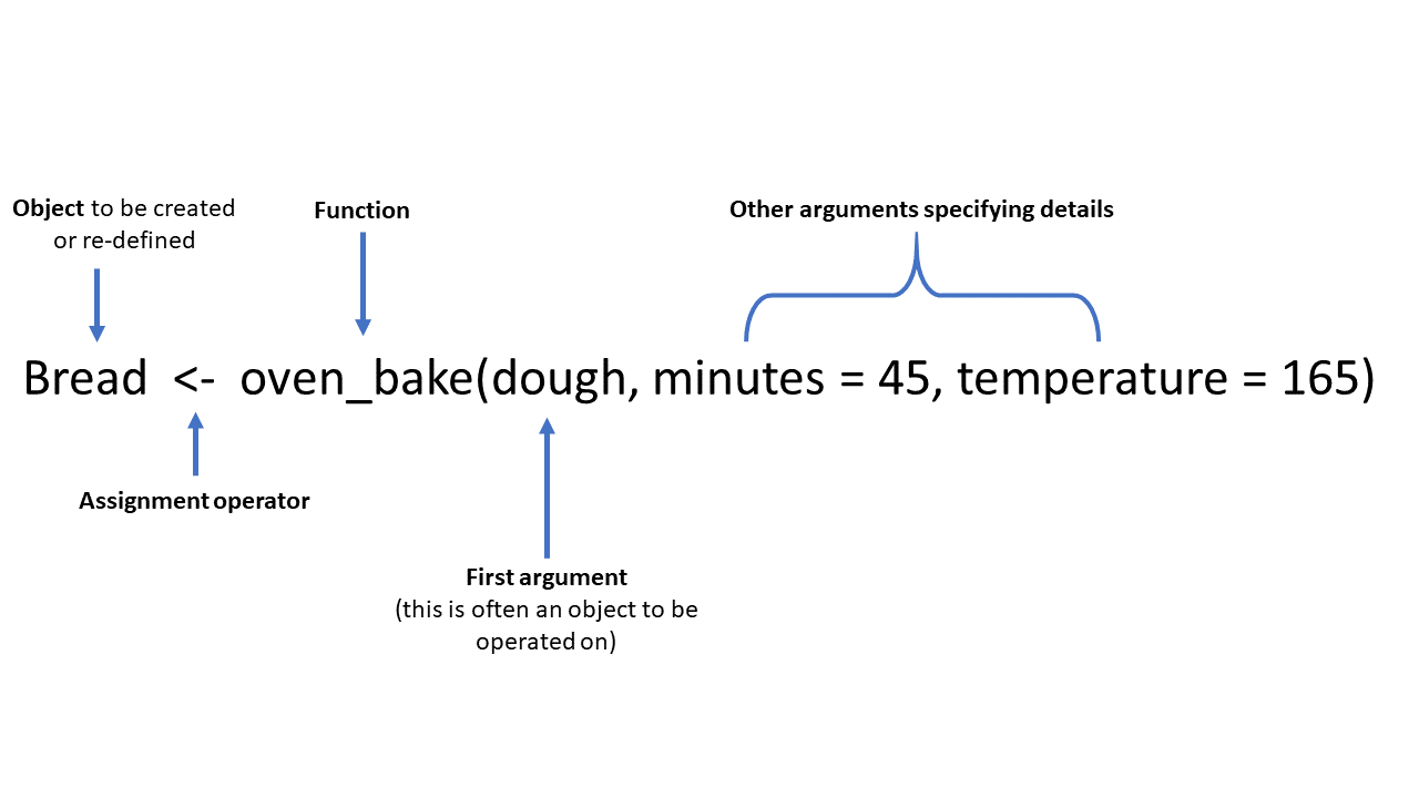
Here is a fun fictional function, called oven_bake(), as an example of a typical function. It takes an input object (e.g. a dataset, or in this example “dough”) and performs operations on it as specified by additional arguments (minutes = and temperature =). The output can be printed to the console, or saved as an object using the assignment operator <-.

In a more realistic example, the age_pyramid() command below produces an age pyramid plot based on defined age groups and a binary split column, such as gender. The function is given three arguments within the parentheses, separated by commas. The values supplied to the arguments establish linelist as the dataframe to use, age_cat5 as the column to count, and gender as the binary column to use for splitting the pyramid by color.

# Create an age pyramid
age_pyramid(data = linelist, age_group = "age_cat5", split_by = "gender")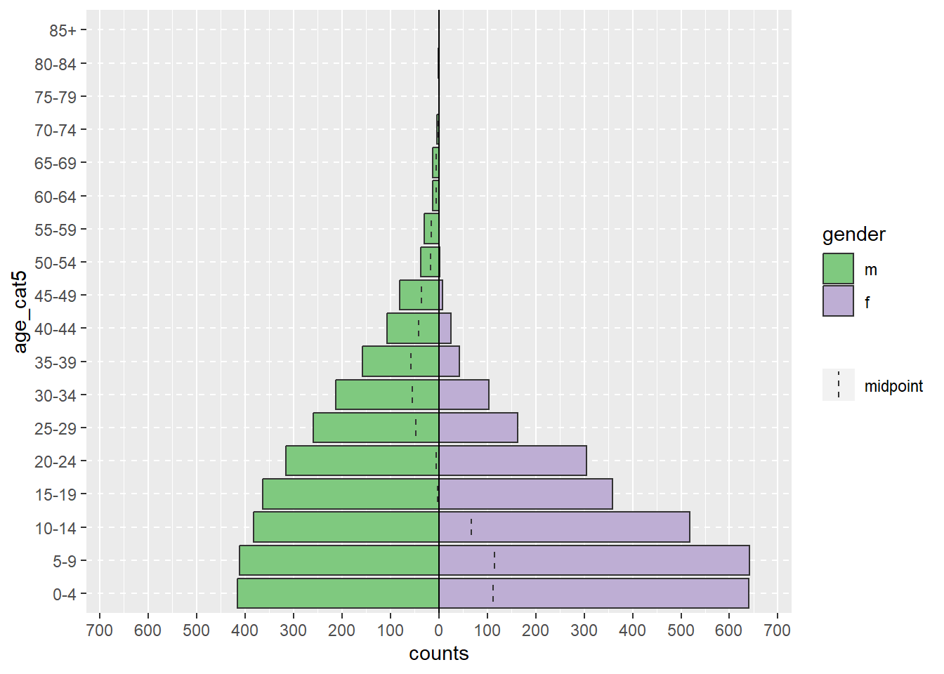

The above command can be equivalently written as below, in a longer style with a new line for each argument. This style can be easier to read, and easier to write “comments” with # to explain each part (commenting extensively is good practice!). To run this longer command you can highlight the entire command and click “Run”, or just place your cursor in the first line and then press the Ctrl and Enter keys simultaneously.

# Create an age pyramid
age_pyramid(
  data = linelist,        # use case linelist
  age_group = "age_cat5", # provide age group column
  split_by = "gender"     # use gender column for two sides of pyramid
  )

The first half of an argument assignment (e.g. data =) does not need to be specified if the arguments are written in a specific order (specified in the function’s documentation). The below code produces the exact same pyramid as above, because the function expects the argument order: data frame, age_group variable, split_by variable.

# This command will produce the exact same graphic as above
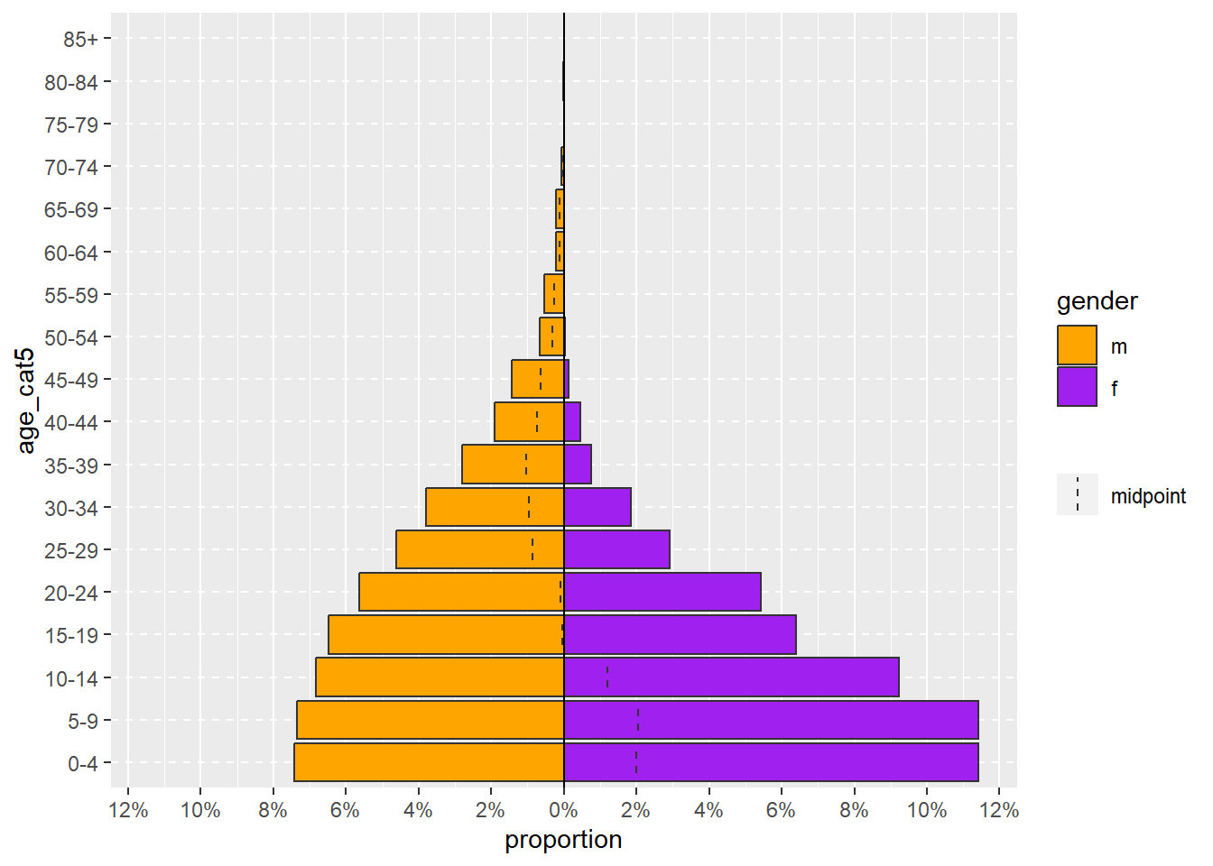
age_pyramid(linelist, "age_cat5", "gender")

A more complex age_pyramid() command might include the optional arguments to:

Show proportions instead of counts (set proportional = TRUE when the default is FALSE)
Specify the two colors to use (pal = is short for “palette” and is supplied with a vector of two color names. See the objects page for how the function c() makes a vector)

Note

For arguments that you specify with both parts of the argument (e.g. proportional = TRUE), their order among all the arguments does not matter.

age_pyramid(
  linelist,                    # use case linelist
  "age_cat5",                  # age group column
  "gender",                    # split by gender
  proportional = TRUE,         # percents instead of counts
  pal = c("orange", "purple")  # colors
  )

Packages

Packages contain functions.

An R package is a shareable bundle of code and documentation that contains pre-defined functions. Users in the R community develop packages all the time catered to specific problems, it is likely that one can help with your work! You will install and use hundreds of packages in your use of R.

On installation, R contains “base” packages and functions that perform common elementary tasks. But many R users create specialized functions, which are verified by the R community and which you can download as a package for your own use. In this handbook, package names are written in bold. One of the more challenging aspects of R is that there are often many functions or packages to choose from to complete a given task.

Install and load

Functions are contained within packages which can be downloaded (“installed”) to your computer from the internet. Once a package is downloaded, it is stored in your “library”. You can then access the functions it contains during your current R session by “loading” the package.

Think of R as your personal library: When you download a package, your library gains a new book of functions, but each time you want to use a function in that book, you must borrow (“load”) that book from your library.

In summary: to use the functions available in an R package, 2 steps must be implemented:

The package must be installed (once), and
The package must be loaded (each R session)

Your library

Your “library” is actually a folder on your computer, containing a folder for each package that has been installed. Find out where R is installed in your computer, and look for a folder called “win-library”. For example: R\win-library\4.0 (the 4.0 is the R version - you’ll have a different library for each R version you’ve downloaded).

You can print the file path to your library by entering .libPaths() (empty parentheses).

Install from CRAN

Most often, R users download packages from CRAN. CRAN (Comprehensive R Archive Network) is an online public warehouse of R packages that have been published by R community members.

How to install and load

The base R function for installing a package is install.packages(). The name of the package to install must be provided in the parentheses in quotes. If you want to install multiple packages in one command, they must be listed within a character vector c().

Common Mistake

This command installs a package, but does not load it for use in the current session.

# install a single package with base R
install.packages("tidyverse")

# install multiple packages with base R
install.packages(c("tidyverse", "rio", "here"))

Installation can also be accomplished point-and-click by going to the RStudio “Packages” pane and clicking “Install” and searching for the desired package name.

The base R function to load a package for use (after it has been installed) is library(). It can load only one package at a time (another reason to use p_load()). You can provide the package name with or without quotes.

# load packages for use, with base R
library(tidyverse)
library(rio)
library(here)

To check whether a package in installed and/or loaded, you can view the Packages pane in RStudio. If the package is installed, it is shown there with version number. If its box is checked, it is loaded for the current session.

Code syntax

For clarity in this handbook, functions are sometimes preceded by the name of their package using the :: symbol in the following way: package_name::function_name()

Once a package is loaded for a session, this explicit style is not necessary. One can just use function_name(). However writing the package name is useful when a function name is common and may exist in multiple packages (e.g. plot()). Writing the package name will also load the package if it is not already loaded.

# This command uses the package "rio" and its function "import()" to import a dataset
linelist <- rio::import("linelist.xlsx", which = "Sheet1")

Function help

To read more about a function, you can search for it in the Help tab of the lower-right RStudio. You can also run a command like ?thefunctionname (put the name of the function after a question mark) and the Help page will appear in the Help pane. Finally, try searching online for resources.

Update packages

You can update packages by re-installing them. You can also click the green “Update” button in your RStudio Packages pane to see which packages have new versions Wto install. Be aware that your old code may need to be updated if there is a major revision to how a function works!

Delete packages

Use remove.packages(). Alternatively, go find the folder which contains your library and manually delete the folder.

Dependencies

Packages often depend on other packages to work. These are called dependencies. If a dependency fails to install, then the package depending on it may also fail to install.

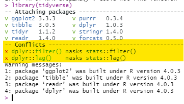
Masked functions

It is not uncommon that two or more packages contain the same function name. For example, the package dplyr has a filter() function, but so does the package stats. The default filter() function depends on the order these packages are first loaded in the R session - the later one will be the default for the command filter().

You can check the order in your Environment pane of R Studio - click the drop-down for “Global Environment” and see the order of the packages. Functions from packages lower on that drop-down list will mask functions of the same name in packages that appear higher in the drop-down list. When first loading a package, R will warn you in the console if masking is occurring, but this can be easy to miss.

Here are ways you can fix masking:

Specify the package name in the command. For example, use dplyr::filter()
Re-arrange the order in which the packages are loaded and start a new R session

Install older version

See this guide to install an older version of a particular package.

Scripts

Scripts are a fundamental part of programming. They are documents that hold your commands (e.g. functions to create and modify datasets, print visualizations, etc). You can save a script and run it again later. There are many advantages to storing and running your commands from a script (vs. typing commands one-by-one into the R console “command line”):

Portability - you can share your work with others by sending them your scripts
Reproducibility - so that you and others know exactly what you did
Version control - so you can track changes made by yourself or colleagues
Commenting/annotation - to explain to your colleagues what you have done

Commenting

In a script you can also annotate (“comment”) around your R code. Commenting is helpful to explain to yourself and other readers what you are doing. You can add a comment by typing the hash symbol (#) and writing your comment after it. The commented text will appear in a different color than the R code.

Any code written after the # will not be run. Therefore, placing a # before code is also a useful way to temporarily block a line of code (“comment out”) if you do not want to delete it). You can comment out/in multiple lines at once by highlighting them and pressing Ctrl+Shift+c (Cmd+Shift+c in Mac).

# A comment can be on a line by itself
# import data
linelist <- import("linelist_raw.xlsx") %>%   # a comment can also come after code
# filter(age > 50)                          # It can also be used to deactivate / remove a line of code
  count()

Comment on what you are doing and on why you are doing it.
Break your code into logical sections
Accompany your code with a text step-by-step description of what you are doing (e.g. numbered steps)

Style

It is important to be conscious of your coding style - especially if working on a team. Some nice R styles guide are the tidyverse style guide, Hadley Wickham’s style guide, and Google’s. There are also packages such as styler and lintr which help you conform to a style.

A few very basic points to make your code readable to others:
* When naming objects, use only lowercase letters, numbers, and underscores _, e.g. my_data
* Use frequent spaces, including around operators, e.g. n = 1 and age_new <- age_old + 3

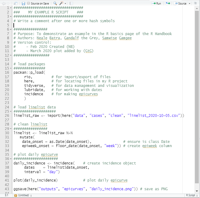
Example Script

Below is an example of a short R script. Remember, the better you succinctly explain your code in comments, the more your colleagues will like you!

Quarto/R markdown

An R markdown script is a type of R script in which the script itself becomes an output document (PDF, Word, HTML, Powerpoint, etc.). Quarto is a new version of R markdown. These are incredibly useful and versatile tools often used to create dynamic and automated reports. Even this website is produced with Quarto!

Objects

Everything in R is an object, and R is an “object-oriented” language. These sections will explain:

How to create objects (<-)
Types of objects (e.g. data frames, vectors..)
How to access subparts of objects (e.g. variables in a dataset)
Classes of objects (e.g. numeric, logical, integer, double, character, factor)

Everything is an object

Everything you store in R - datasets, variables, a list of village names, a total population number, even outputs such as graphs - are objects which are assigned a name and can be referenced in later commands.

An object exists when you have assigned it a value (see the assignment section below). When it is assigned a value, the object appears in the Environment (see the upper right pane of RStudio). It can then be operated upon, manipulated, changed, and re-defined.

Defining objects (`<-`)

Create objects by assigning them a value with the <- operator.
You can think of the assignment operator <- as the words “is defined as”. Assignment commands generally follow a standard order:

object_name <- value (or process/calculation that produce a value)

For example, you may want to record the current epidemiological reporting week as an object for reference in later code. In this example, the object current_week is created when it is assigned the value "2018-W10" (the quote marks make this a character value). The object current_week will then appear in the RStudio Environment pane (upper-right) and can be referenced in later commands.

See the R commands and their output in the boxes below.

current_week <- "2018-W10"   # this command creates the object current_week by assigning it a value
current_week                 # this command prints the current value of current_week object in the console

[1] "2018-W10"

Note

Note the [1] in the R console output is simply indicating that you are viewing the first item of the output

Common Mistake

An object’s value can be over-written at any time by running an assignment command to re-define its value. Thus, the order of the commands run is very important.

For instance, the following command will re-define the value of current_week:

current_week <- "2018-W51"   # assigns a NEW value to the object current_week
current_week                 # prints the current value of current_week in the console

[1] "2018-W51"

Equals signs =

You will also see equals signs in R code:

A double equals sign == between two objects or values asks a logical question: “is this equal to that?”.
You will also see equals signs within functions used to specify values of function arguments (read about these in sections below), for example max(age, na.rm = TRUE).
You can use a single equals sign = in place of <- to create and define objects, but this is discouraged. You can read about why this is discouraged here.

Datasets

Datasets are also objects (typically “dataframes”) and must be assigned names when they are imported. In the code below, the object linelist is created and assigned the value of a CSV file imported with the rio package and its import() function.

# linelist is created and assigned the value of the imported CSV file
linelist <- import("my_linelist.csv")

Naming Objects

Object names must not contain spaces, but you should use underscore (_) or a period (.) instead of a space.
Object names are case-sensitive (meaning that Dataset_A is different from dataset_A).
Object names must begin with a letter (cannot begin with a number like 1, 2 or 3).

Outputs

Outputs like tables and plots provide an example of how outputs can be saved as objects, or just be printed without being saved. A cross-tabulation of gender and outcome using the base R function table() can be printed directly to the R console (without being saved).

# printed to R console only
table(linelist$gender, linelist$outcome)

   
    Death Recover
  f  1227     953
  m  1228     950

But the same table can be saved as a named object. Then, optionally, it can be printed.

# save
gen_out_table <- table(linelist$gender, linelist$outcome)

# print
gen_out_table

   
    Death Recover
  f  1227     953
  m  1228     950

Columns

Columns in a dataset are also objects and can be defined, over-written, and created as described below in the section on Columns.

You can use the assignment operator from base R to create a new column. Below, the new column bmi (Body Mass Index) is created, and for each row the new value is result of a mathematical operation on the row’s value in the wt_kg and ht_cm columns.

# create new "bmi" column using base R syntax
linelist$bmi <- linelist$wt_kg / (linelist$ht_cm/100)^2

However, in this handbook, we emphasize a different approach to defining columns, which uses the function mutate() from the dplyr package and piping with the pipe operator (%>%). The syntax is easier to read and there are other advantages.

# create new "bmi" column using dplyr syntax
linelist <- linelist %>% 
  mutate(bmi = wt_kg / (ht_cm/100)^2)

Object structure

Objects can be a single piece of data (e.g. my_number <- 24), or they can consist of structured data.

The graphic below is borrowed from this online R tutorial. It shows some common data structures and their names.

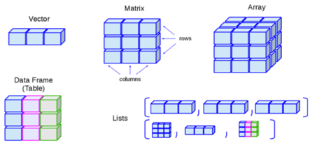
In epidemiology (and particularly field epidemiology), you will most commonly encounter data frames and vectors:

Common structure	Explanation	Example
Vectors	A container for a sequence of singular objects, all of the same class (e.g. numeric, character).	“Variables” (columns) in data frames are vectors (e.g. the column `age_years`).
Data Frames	Vectors (e.g. columns) that are bound together that all have the same number of rows.	`linelist` is a data frame.

Note that to create a vector that “stands alone” (is not part of a data frame) the function c() is used to combine the different elements. For example, if creating a vector of colors plot’s color scale: vector_of_colors <- c("blue", "red2", "orange", "grey")

Object classes

All the objects stored in R have a class which tells R how to handle the object. There are many possible classes, but common ones include:

Class	Explanation	Examples
Character	These are text/words/sentences “within quotation marks”. Math cannot be done on these objects.	“Character objects are in quotation marks”
Integer	Numbers that are whole only (no decimals)	-5, 14, or 2000
Numeric	These are numbers and can include decimals. If within quotation marks they will be considered character class.	23.1 or 14
Factor	These are vectors that have a specified order or hierarchy of values	An variable of economic status with ordered values
Date	Once R is told that certain data are Dates, these data can be manipulated and displayed in special ways.	2018-04-12 or 15/3/1954 or Wed 4 Jan 1980
Logical	Values must be one of the two special values TRUE or FALSE (note these are not “TRUE” and “FALSE” in quotation marks)	TRUE or FALSE
data.frame	A data frame is how R stores a typical dataset. It consists of vectors (columns) of data bound together, that all have the same number of observations (rows).	The example AJS dataset named `linelist_raw` contains 68 variables with 300 observations (rows) each.
tibble	tibbles are a variation on data frame, the main operational difference being that they print more nicely to the console (display first 10 rows and only columns that fit on the screen)	Any data frame, list, or matrix can be converted to a tibble with `as_tibble()`
list	A list is like vector, but holds other objects that can be other different classes	A list could hold a single number, and a dataframe, and a vector, and even another list within it!

You can test the class of an object by providing its name to the function class(). You can reference a specific column within a dataset using the $ notation to separate the name of the dataset and the name of the column.

class(linelist)         # class should be a data frame or tibble

[1] "data.frame"

class(linelist$age)     # class should be numeric

[1] "numeric"

class(linelist$gender)  # class should be character

[1] "character"

Sometimes, a column will be converted to a different class automatically by R. Watch out for this! For example, if you have a vector or column of numbers, but a character value is inserted… the entire column will change to class character.

num_vector <- c(1,2,3,4,5) # define vector as all numbers
class(num_vector)          # vector is numeric class

[1] "numeric"

num_vector[3] <- "three"   # convert the third element to a character
class(num_vector)          # vector is now character class

[1] "character"

One common example of this is when manipulating a data frame in order to print a table - if you make a total row and try to paste/glue together percents in the same cell as numbers (e.g. 23 (40%)), the entire numeric column above will convert to character and can no longer be used for mathematical calculations.Sometimes, you will need to convert objects or columns to another class.

Function	Action
`as.character()`	Converts to character class
`as.numeric()`	Converts to numeric class
`as.integer()`	Converts to integer class
`as.Date()`	Converts to Date class
`factor()`	Converts to factor

Likewise, there are base R functions to check whether an object IS of a specific class, such as is.numeric(), is.character(), is.double(), is.factor(), is.integer()

Here is more online material on classes and data structures in R.

Columns/Variables (`$`)

A column in a data frame is technically a “vector” (see table above) - a series of values that must all be the same class (either character, numeric, logical, etc).

A vector can exist independent of a data frame, for example a vector of column names that you want to include as explanatory variables in a model. To create a “stand alone” vector, use the c() function as below:

# define the stand-alone vector of character values
explanatory_vars <- c("gender", "fever", "chills", "cough", "aches", "vomit")

# print the values in this named vector
explanatory_vars

[1] "gender" "fever"  "chills" "cough"  "aches"  "vomit"

Columns in a data frame are also vectors and can be called, referenced, extracted, or created using the $ symbol. The $ symbol connects the name of the column to the name of its data frame. In this handbook, we try to use the word “column” instead of “variable”.

# Retrieve the length of the vector age_years
length(linelist$age) # (age is a column in the linelist data frame)

Access/index with brackets (`[ ]`)

You may need to view parts of objects, also called “indexing”, which is often done using the square brackets [ ]. Using $ on a dataframe to access a column is also a type of indexing.

my_vector <- c("a", "b", "c", "d", "e", "f")  # define the vector
my_vector[5]                                  # print the 5th element

[1] "e"

Square brackets also work to return specific parts of an returned output, such as the output of a summary() function:

# All of the summary
summary(linelist$age)

   Min. 1st Qu.  Median    Mean 3rd Qu.    Max.    NA's 
   0.00    6.00   13.00   16.07   23.00   84.00      86

# Just the second element of the summary, with name (using only single brackets)
summary(linelist$age)[2]

1st Qu. 
      6

# Just the second element, without name (using double brackets)
summary(linelist$age)[[2]]

[1] 6

# Extract an element by name, without showing the name
summary(linelist$age)[["Median"]]

[1] 13

Brackets also work on data frames to view specific rows and columns. You can do this using the syntax dataframe[rows, columns]:

# View a specific row (2) from dataset, with all columns (don't forget the comma!)
linelist[2,]

# View all rows, but just one column
linelist[, "date_onset"]

# View values from row 2 and columns 5 through 10
linelist[2, 5:10] 

# View values from row 2 and columns 5 through 10 and 18
linelist[2, c(5:10, 18)] 

# View rows 2 through 20, and specific columns
linelist[2:20, c("date_onset", "outcome", "age")]

# View rows and columns based on criteria
# *** Note the dataframe must still be named in the criteria!
linelist[linelist$age > 25 , c("date_onset", "outcome", "age")]

# Use View() to see the outputs in the RStudio Viewer pane (easier to read) 
# *** Note the capital "V" in View() function
View(linelist[2:20, "date_onset"])

# Save as a new object
new_table <- linelist[2:20, c("date_onset")]

Using Tidyverse Instead

In a future session, we will learn how to perform many of these operations using dplyr syntax (functions filter() for rows, and select() for columns) as opposed to the base R syntax shown here.

To filter based on “row number”, you can use the dplyr function row_number() with open parentheses as part of a logical filtering statement. Often you will use the %in% operator and a range of numbers as part of that logical statement, as shown below. To see the first N rows, you can also use the special dplyr function head().

# View first 100 rows
linelist %>% head(100)

# Show row 5 only
linelist %>% filter(row_number() == 5)

# View rows 2 through 20, and three specific columns (note no quotes necessary on column names)
linelist %>% filter(row_number() %in% 2:20) %>% select(date_onset, outcome, age)

When indexing an object of class list, single brackets always return with class list, even if only a single object is returned. Double brackets, however, can be used to access a single element and return a different class than list.
Brackets can also be written after one another, as demonstrated below.

This visual explanation of lists indexing, with pepper shakers is humorous and helpful.

# define demo list
my_list <- list(
  # First element in the list is a character vector
  hospitals = c("Central", "Empire", "Santa Anna"),
  
  # second element in the list is a data frame of addresses
  addresses   = data.frame(
    street = c("145 Medical Way", "1048 Brown Ave", "999 El Camino"),
    city   = c("Andover", "Hamilton", "El Paso")
    )
  )

Here is how the list looks when printed to the console. See how there are two named elements:

hospitals, a character vector
addresses, a data frame of addresses

my_list

$hospitals
[1] "Central"    "Empire"     "Santa Anna"

$addresses
           street     city
1 145 Medical Way  Andover
2  1048 Brown Ave Hamilton
3   999 El Camino  El Paso

Now we extract, using various methods:

my_list[1] # this returns the element in class "list" - the element name is still displayed

$hospitals
[1] "Central"    "Empire"     "Santa Anna"

my_list[[1]] # this returns only the (unnamed) character vector

[1] "Central"    "Empire"     "Santa Anna"

my_list[["hospitals"]] # you can also index by name of the list element

[1] "Central"    "Empire"     "Santa Anna"

my_list[[1]][3] # this returns the third element of the "hospitals" character vector

[1] "Santa Anna"

my_list[[2]][1] # This returns the first column ("street") of the address data frame

           street
1 145 Medical Way
2  1048 Brown Ave
3   999 El Camino

Remove objects

You can remove individual objects from your R environment by putting the name in the rm() function (no quote marks):

rm(object_name)

You can remove all objects (clear your workspace) by running:

rm(list = ls(all = TRUE))

Categorical data: factors

Since factors are special vectors, the same rules for selecting values using indices apply.

expression <- c("high","low","low","medium","high","medium","medium","low","low","low")

The elements of this expression factor created previously has following categories or levels: low, medium, and high.

Let’s extract the values of the factor with high expression, and let’s using nesting here:

expression[expression == "high"]    ## This will only return those elements in the factor equal to "high"

[1] "high" "high"

Nesting note:

The piece of code above was more efficient with nesting; we used a single step instead of two steps as shown below:

Step1 (no nesting): idx <- expression == "high"

Step2 (no nesting): expression[idx]

Releveling factors

We have briefly talked about factors, but this data type only becomes more intuitive once you’ve had a chance to work with it. Let’s take a slight detour and learn about how to relevel categories within a factor.

To view the integer assignments under the hood you can use str():

expression

 [1] "high"   "low"    "low"    "medium" "high"   "medium" "medium" "low"   
 [9] "low"    "low"

The categories are referred to as “factor levels”. As we learned earlier, the levels in the expression factor were assigned integers alphabetically, with high=1, low=2, medium=3. However, it makes more sense for us if low=1, medium=2 and high=3, i.e. it makes sense for us to “relevel” the categories in this factor.

To relevel the categories, you can add the levels argument to the factor() function, and give it a vector with the categories listed in the required order:

expression <- factor(expression, levels=c("low", "medium", "high"))     # you can re-factor a factor

Now we have a releveled factor with low as the lowest or first category, medium as the second and high as the third. This is reflected in the way they are listed in the output of str(), as well as in the numbering of which category is where in the factor.

Note: Releveling becomes necessary when you need a specific category in a factor to be the “base” category, i.e. category that is equal to 1. One example would be if you need the “control” to be the “base” in a given RNA-seq experiment.

Piping (`%>%`)

Two general approaches to working with objects are:

Pipes/tidyverse - pipes send an object from function to function - emphasis is on the action, not the object
Define intermediate objects - an object is re-defined again and again - emphasis is on the object

Pipes

Simply explained, the pipe operator (%>%) passes an intermediate output from one function to the next.
You can think of it as saying “then”. Many functions can be linked together with %>%.

Piping emphasizes a sequence of actions, not the object the actions are being performed on
Pipes are best when a sequence of actions must be performed on one object
Pipes come from the package magrittr, which is automatically included in packages dplyr and tidyverse
Pipes can make code more clean and easier to read, more intuitive

Read more on this approach in the tidyverse style guide

Here is a fake example for comparison, using fictional functions to “bake a cake”. First, the pipe method:

# A fake example of how to bake a cake using piping syntax

cake <- flour %>%       # to define cake, start with flour, and then...
  add(eggs) %>%   # add eggs
  add(oil) %>%    # add oil
  add(water) %>%  # add water
  mix_together(         # mix together
    utensil = spoon,
    minutes = 2) %>%    
  bake(degrees = 350,   # bake
       system = "fahrenheit",
       minutes = 35) %>%  
  let_cool()            # let it cool down

Here is another link describing the utility of pipes.

Piping is not a base function. To use piping, the magrittr package must be installed and loaded (this is typically done by loading tidyverse or dplyr package which include it). You can read more about piping in the magrittr documentation.

Note that just like other R commands, pipes can be used to just display the result, or to save/re-save an object, depending on whether the assignment operator <- is involved. See both below:

# Create or overwrite object, defining as aggregate counts by age category (not printed)
linelist_summary <- linelist %>% 
  count(age_cat)

# Print the table of counts in the console, but don't save it
linelist %>% 
  count(age_cat)

  age_cat    n
1     0-4 1095
2     5-9 1095
3   10-14  941
4   15-19  743
5   20-29 1073
6   30-49  754
7   50-69   95
8     70+    6
9    <NA>   86

%<>%
This is an “assignment pipe” from the magrittr package, which pipes an object forward and also re-defines the object. It must be the first pipe operator in the chain. It is shorthand. The below two commands are equivalent:

linelist <- linelist %>%
  filter(age > 50)

linelist %<>% filter(age > 50)

Define intermediate objects

This approach to changing objects/dataframes may be better if:

You need to manipulate multiple objects
There are intermediate steps that are meaningful and deserve separate object names

Risks:

Creating new objects for each step means creating lots of objects. If you use the wrong one you might not realize it!
Naming all the objects can be confusing
Errors may not be easily detectable

Either name each intermediate object, or overwrite the original, or combine all the functions together. All come with their own risks.

Below is the same fake “cake” example as above, but using this style:

# a fake example of how to bake a cake using this method (defining intermediate objects)
batter_1 <- left_join(flour, eggs)
batter_2 <- left_join(batter_1, oil)
batter_3 <- left_join(batter_2, water)

batter_4 <- mix_together(object = batter_3, utensil = spoon, minutes = 2)

cake <- bake(batter_4, degrees = 350, system = "fahrenheit", minutes = 35)

cake <- let_cool(cake)

Combine all functions together - this is difficult to read:

# an example of combining/nesting mutliple functions together - difficult to read
cake <- let_cool(bake(mix_together(batter_3, utensil = spoon, minutes = 2), degrees = 350, system = "fahrenheit", minutes = 35))

Errors vs. warnings and debugging tips

Error versus Warning

When a command is run, the R Console may show you warning or error messages in red text.

A warning means that R has completed your command, but had to take additional steps or produced unusual output that you should be aware of.
An error means that R was not able to complete your command.

Look for clues:

The error/warning message will often include a line number for the problem.
If an object “is unknown” or “not found”, perhaps you spelled it incorrectly, forgot to call a package with library(), or forgot to re-run your script after making changes.

If all else fails, copy the error message into Google along with some key terms - chances are that someone else has worked through this already!

General syntax tips

A few things to remember when writing commands in R, to avoid errors and warnings:

Always close parentheses - tip: count the number of opening “(” and closing parentheses “)” for each code chunk
Avoid spaces in column and object names. Use underscore ( _ ) or periods ( . ) instead
Keep track of and remember to separate a function’s arguments with commas

Code assists

Any script (RMarkdown or otherwise) will give clues when you have made a mistake. For example, if you forgot to write a comma where it is needed, or to close a parentheses, RStudio will raise a flag on that line, on the right side of the script, to warn you.

R Basics

Functions

Simple functions

Functions with multiple arguments

Packages

Install and load

Your library

Install from CRAN

How to install and load

Code syntax

Function help

Update packages

Delete packages

Dependencies

Masked functions

Install older version

Scripts

Commenting

Style

Example Script

Quarto/R markdown

Objects

Everything is an object

Defining objects (<-)

Object structure

Object classes

Columns/Variables ($)

Access/index with brackets ([ ])

Remove objects

Categorical data: factors

Releveling factors

Piping (%>%)

Pipes

Define intermediate objects

Errors vs. warnings and debugging tips

Error versus Warning

General syntax tips

Code assists

Defining objects (`<-`)

Columns/Variables (`$`)

Access/index with brackets (`[ ]`)

Piping (`%>%`)