Core Data Functions

Extended Materials

You can find the original, extended version of this chapter here.

Data Preparation

pacman::p_load(
  rio,        # importing data  
  here,       # relative file pathways  
  janitor,    # data cleaning and tables
  lubridate,  # working with dates
  matchmaker, # dictionary-based cleaning
  epikit,     # age_categories() function
  tidyverse   # data management and visualization
)
linelist <- rio::import("data/case_linelists/linelist_cleaned.rds")

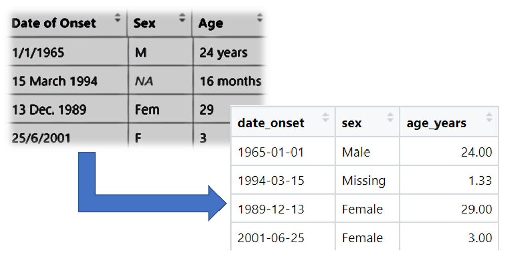
This week we are going to learn how to use R to manipulate data. This will include learning about core functions for manipulating and summarizing data, as well as using conditional statements to create subsets.

Key operators, functions, and constants

An operators is a symbol or set of symbols representing some mathematical or logical operation. They are essentially equivalent to functions. R has a number of built-in operators, and libraries may add additional operators (such as the %>% operator used in Tidyverse packages). Some examples of operators are:

Definitional operators
Relational operators (less than, equal too..)
Logical operators (and, or…)
Handling missing values
Mathematical operators and functions (+/-, >, sum(), median(), …)
The %in% operator

R also has some built-in constants, which have the same meaning in programming as in mathematics and statistics. Examples of constants in R include:

pi which in base R equals 3.141593
Inf and -Inf for positive and negative infinity
NaN for not a number (such as the result of 0/0)
NA for missing data

Assignment operators

<-

The basic assignment operator in R is <-. Such that object_name <- value.
This assignment operator can also be written as =. We advise use of <- for general R use.
We also advise surrounding such operators with spaces, for readability.

Relational and logical operators

Relational operators compare values and are often used when defining new variables and subsets of datasets. Here are the common relational operators in R:

Meaning	Operator	Example	Example Result
Equal to	`==`	`"A" == "a"`	`FALSE` (because R is case sensitive) Note that == (double equals) is different from = (single equals), which acts like the assignment operator `<-`
Not equal to	`!=`	`2 != 0`	`TRUE`
Greater than	`>`	`4 > 2`	`TRUE`
Less than	`<`	`4 < 2`	`FALSE`
Greater than or equal to	`>=`	`6 >= 4`	`TRUE`
Less than or equal to	`<=`	`6 <= 4`	`FALSE`
Value is missing	`is.na()`	`is.na(7)`	`FALSE`
Value is not missing	`!is.na()`	`!is.na(7)`	`TRUE`

Logical operators, such as AND and OR, are often used to connect relational operators and create more complicated criteria. Complex statements might require parentheses ( ) for grouping and order of application.

Meaning	Operator
AND	`&`
OR	`\|` (vertical bar)
Parentheses	`( )` Used to group criteria together and clarify order of operations

For example, below, we have a linelist with two variables we want to use to create our case definition, hep_e_rdt, a test result and other_cases_in_hh, which will tell us if there are other cases in the household. The command below uses the function case_when() to create the new variable case_def such that:

linelist_cleaned <- linelist %>%
  mutate(case_def = case_when(
    is.na(rdt_result) & is.na(other_case_in_home)            ~ NA_character_,
    rdt_result == "Positive"                                 ~ "Confirmed",
    rdt_result != "Positive" & other_cases_in_home == "Yes"  ~ "Probable",
    TRUE                                                     ~ "Suspected"
  ))

Criteria in example above	Resulting value in new variable “case_def”
If the value for variables `rdt_result` and `other_cases_in_home` are missing	`NA` (missing)
If the value in `rdt_result` is “Positive”	“Confirmed”
If the value in `rdt_result` is NOT “Positive” AND the value in `other_cases_in_home` is “Yes”	“Probable”
If one of the above criteria are not met	“Suspected”

Note that R is case-sensitive, so “Positive” is different than “positive”…

Missing values

In R, missing values are represented by the special value NA (a “reserved” value) (capital letters N and A - not in quotation marks). To test whether a value is NA, use the special function is.na(), which returns TRUE or FALSE.

rdt_result <- c("Positive", "Suspected", "Positive", NA)   # two positive cases, one suspected, and one unknown
is.na(rdt_result)  # Tests whether the value of rdt_result is NA

[1] FALSE FALSE FALSE  TRUE

We will be learning more about how to deal with missing data in future weeks.

Mathematics and statistics

All the operators and functions in this page are automatically available using base R.

Mathematical operators

These are often used to perform addition, division, to create new columns, etc. Below are common mathematical operators in R. Whether you put spaces around the operators is not important.

Purpose	Example in R
addition	2 + 3
subtraction	2 - 3
multiplication	2 * 3
division	30 / 5
exponent	2^3
order of operations	( )

Mathematical functions

Purpose	Function
rounding	round(x, digits = n)
rounding	janitor::round_half_up(x, digits = n)
ceiling (round up)	ceiling(x)
floor (round down)	floor(x)
absolute value	abs(x)
square root	sqrt(x)
exponent	exponent(x)
natural logarithm	log(x)
log base 10	log10(x)
log base 2	log2(x)

Note: for round() the digits = specifies the number of decimal placed. Use signif() to round to a number of significant figures.

Statistical functions

Warning

The functions below will by default include missing values in calculations. Missing values will result in an output of NA, unless the argument na.rm = TRUE is specified. This can be written shorthand as na.rm = T.

Objective	Function
mean (average)	mean(x, na.rm=T)
median	median(x, na.rm=T)
standard deviation	sd(x, na.rm=T)
quantiles*	quantile(x, probs)
sum	sum(x, na.rm=T)
minimum value	min(x, na.rm=T)
maximum value	max(x, na.rm=T)
range of numeric values	range(x, na.rm=T)
summary**	summary(x)

Notes:

*quantile(): x is the numeric vector to examine, and probs = is a numeric vector with probabilities within 0 and 1.0, e.g c(0.5, 0.8, 0.85)
**summary(): gives a summary on a numeric vector including mean, median, and common percentiles

Warning

If providing a vector of numbers to one of the above functions, be sure to wrap the numbers within c() .}

# If supplying raw numbers to a function, wrap them in c()
mean(1, 6, 12, 10, 5, 0)    # !!! INCORRECT !!!

[1] 1

mean(c(1, 6, 12, 10, 5, 0)) # CORRECT

[1] 5.666667

Other useful functions

Objective	Function	Example
create a sequence	seq(from, to, by)	`seq(1, 10, 2)`
repeat x, n times	rep(x, ntimes)	`rep(1:3, 2)` or `rep(c("a", "b", "c"), 3)`
subdivide a numeric vector	cut(x, n)	`cut(linelist$age, 5)`
take a random sample	sample(x, size)	`sample(linelist$id, size = 5, replace = TRUE)`

`%in%`

A very useful operator for matching values, and for quickly assessing if a value is within a vector or dataframe.

my_vector <- c("a", "b", "c", "d")

"a" %in% my_vector

[1] TRUE

"h" %in% my_vector

[1] FALSE

To ask if a value is not %in% a vector, put an exclamation mark (!) in front of the logic statement:

# to negate, put an exclamation in front
!"a" %in% my_vector

[1] FALSE

!"h" %in% my_vector

[1] TRUE

%in% is very useful when using the dplyr function case_when(). You can define a vector previously, and then reference it later. For example:

affirmative <- c("1", "Yes", "YES", "yes", "y", "Y", "oui", "Oui", "Si")

linelist <- linelist %>% 
  mutate(child_hospitaled = case_when(
    hospitalized %in% affirmative & age < 18 ~ "Hospitalized Child",
    TRUE                                      ~ "Not"))

Tidyverse functions

We will be emphasizing use of the functions from the tidyverse family of R packages. The functions we will be learning about are listed below.

Many of these functions belong to the dplyr R package, which provides “verb” functions to solve data manipulation challenges (the name is a reference to a “data frame-plier. dplyr is part of the tidyverse family of R packages (which also includes ggplot2, tidyr, stringr, tibble, purrr, magrittr, and forcats among others).

Function	Utility	Package
`%>%`	“pipe” (pass) data from one function to the next	magrittr
`mutate()`	create, transform, and re-define columns	dplyr
`select()`	keep, remove, select, or re-name columns	dplyr
`rename()`	rename columns	dplyr
`clean_names()`	standardize the syntax of column names	janitor
`as.character()`, `as.numeric()`, `as.Date()`, etc.	convert the class of a column	base R
`across()`	transform multiple columns at one time	dplyr
tidyselect functions	use logic to select columns	tidyselect
`filter()`	keep certain rows	dplyr
`distinct()`	de-duplicate rows	dplyr
`rowwise()`	operations by/within each row	dplyr
`add_row()`	add rows manually	tibble
`arrange()`	sort rows	dplyr
`recode()`	re-code values in a column	dplyr
`case_when()`	re-code values in a column using more complex logical criteria	dplyr
`replace_na()`, `na_if()`, `coalesce()`	special functions for re-coding	tidyr
`age_categories()` and `cut()`	create categorical groups from a numeric column	epikit and base R
`match_df()`	re-code/clean values using a data dictionary	matchmaker
`which()`	apply logical criteria; return indices	base R