Descriptive analysis

This page demonstrates the use of janitor, dplyr, and base R to summarise data and create tables with descriptive statistics.

Here we’ll learn how to create the underlying tables, whereas in the next chapter we’ll see how to nicely format and print them.

Data Preparation

Load packages

pacman::p_load(
  rio,          # File import
  here,         # File locator
  skimr,        # get overview of data
  tidyverse,    # data management + ggplot2 graphics 
  gtsummary,    # summary statistics and tests
  janitor,      # adding totals and percents to tables
  scales,       # easily convert proportions to percents  
  flextable     # converting tables to pretty images
  )

Import data

We import the dataset of cases from a simulated Ebola epidemic. If you want to follow along, click to download the “clean” linelist (as .rds file).

# import the linelist
linelist <- import("linelist_cleaned.rds")

Browse data

Summary statistics

You can use base R functions to return summary statistics on a numeric column. You can return most of the useful summary statistics for a numeric column using summary(), as below. Note that the data frame name must also be specified as shown below.

summary(linelist$age_years)

   Min. 1st Qu.  Median    Mean 3rd Qu.    Max.    NA's 
   0.00    6.00   13.00   16.02   23.00   84.00      86

You can access and save one specific part of it with index brackets [ ]:

summary(linelist$age_years)[[2]]            # return only the 2nd element

[1] 6

# equivalent, alternative to above by element name
# summary(linelist$age_years)[["1st Qu."]]

You can return individual statistics with base R functions like max(), min(), median(), mean(), quantile(), sd(), and range().

Warning

If your data contain missing values, R wants you to know this and so will return NA unless you specify to the above mathematical functions that you want R to ignore missing values, via the argument na.rm = TRUE.

janitor package

The janitor packages offers the tabyl() function to produce tabulations and cross-tabulations, which can be “adorned” or modified with helper functions to display percents, proportions, counts, etc.

Below, we pipe the linelist data frame to janitor functions and print the result. If desired, you can also save the resulting tables with the assignment operator <-.

Simple tabyl

The default use of tabyl() on a specific column produces the unique values, counts, and column-wise “percents” (actually proportions). The proportions may have many digits. You can adjust the number of decimals with adorn_rounding() as described below.

linelist %>% tabyl(age_cat)

 age_cat    n     percent valid_percent
     0-4 1095 0.185971467   0.188728025
     5-9 1095 0.185971467   0.188728025
   10-14  941 0.159816576   0.162185453
   15-19  743 0.126188859   0.128059290
   20-29 1073 0.182235054   0.184936229
   30-49  754 0.128057065   0.129955188
   50-69   95 0.016134511   0.016373664
     70+    6 0.001019022   0.001034126
    <NA>   86 0.014605978            NA

As you can see above, if there are missing values they display in a row labeled <NA>. You can suppress them with show_na = FALSE. If there are no missing values, this row will not appear. If there are missing values, all proportions are given as both raw (denominator inclusive of NA counts) and “valid” (denominator excludes NA counts).

If the column is class Factor and only certain levels are present in your data, all levels will still appear in the table. You can suppress this feature by specifying show_missing_levels = FALSE.

Cross-tabulation

Cross-tabulation counts are achieved by adding one or more additional columns within tabyl(). Note that now only counts are returned - proportions and percents can be added with additional steps shown below.

linelist %>% tabyl(age_cat, gender)

 age_cat   f   m NA_
     0-4 640 416  39
     5-9 641 412  42
   10-14 518 383  40
   15-19 359 364  20
   20-29 468 575  30
   30-49 179 557  18
   50-69   2  91   2
     70+   0   5   1
    <NA>   0   0  86

“Adorning” the tabyl

Use janitor’s “adorn” functions to add totals or convert to proportions, percents, or otherwise adjust the display. Often, you will pipe the tabyl through several of these functions.

Function	Outcome
`adorn_totals()`	Adds totals (`where =` “row”, “col”, or “both”). Set `name =` for “Total”.
`adorn_percentages()`	Convert counts to proportions, with `denominator =` “row”, “col”, or “all”
`adorn_pct_formatting()`	Converts proportions to percents. Specify `digits =`. Remove the “%” symbol with `affix_sign = FALSE`.
`adorn_rounding()`	To round proportions to `digits =` places. To round percents use `adorn_pct_formatting()` with `digits =`.
`adorn_ns()`	Add counts to a table of proportions or percents. Indicate `position =` “rear” to show counts in parentheses, or “front” to put the percents in parentheses.
`adorn_title()`	Add string via arguments `row_name =` and/or `col_name =`

Be conscious of the order you apply the above functions. Below are some examples.

A simple one-way table with percents instead of the default proportions.

linelist %>%               # case linelist
  tabyl(age_cat) %>%       # tabulate counts and proportions by age category
  adorn_pct_formatting()   # convert proportions to percents

 age_cat    n percent valid_percent
     0-4 1095   18.6%         18.9%
     5-9 1095   18.6%         18.9%
   10-14  941   16.0%         16.2%
   15-19  743   12.6%         12.8%
   20-29 1073   18.2%         18.5%
   30-49  754   12.8%         13.0%
   50-69   95    1.6%          1.6%
     70+    6    0.1%          0.1%
    <NA>   86    1.5%             -

A cross-tabulation with a total row and row percents.

linelist %>%                                  
  tabyl(age_cat, gender) %>%                  # counts by age and gender
  adorn_totals(where = "row") %>%             # add total row
  adorn_percentages(denominator = "row") %>%  # convert counts to proportions
  adorn_pct_formatting(digits = 1)            # convert proportions to percents

 age_cat     f     m    NA_
     0-4 58.4% 38.0%   3.6%
     5-9 58.5% 37.6%   3.8%
   10-14 55.0% 40.7%   4.3%
   15-19 48.3% 49.0%   2.7%
   20-29 43.6% 53.6%   2.8%
   30-49 23.7% 73.9%   2.4%
   50-69  2.1% 95.8%   2.1%
     70+  0.0% 83.3%  16.7%
    <NA>  0.0%  0.0% 100.0%
   Total 47.7% 47.6%   4.7%

A cross-tabulation adjusted so that both counts and percents are displayed.

linelist %>%                                  # case linelist
  tabyl(age_cat, gender) %>%                  # cross-tabulate counts
  adorn_totals(where = "row") %>%             # add a total row
  adorn_percentages(denominator = "col") %>%  # convert to proportions
  adorn_pct_formatting() %>%                  # convert to percents
  adorn_ns(position = "front") %>%            # display as: "count (percent)"
  adorn_title(                                # adjust titles
    row_name = "Age Category",
    col_name = "Gender")

                      Gender                            
 Age Category              f              m          NA_
          0-4   640  (22.8%)   416  (14.8%)  39  (14.0%)
          5-9   641  (22.8%)   412  (14.7%)  42  (15.1%)
        10-14   518  (18.5%)   383  (13.7%)  40  (14.4%)
        15-19   359  (12.8%)   364  (13.0%)  20   (7.2%)
        20-29   468  (16.7%)   575  (20.5%)  30  (10.8%)
        30-49   179   (6.4%)   557  (19.9%)  18   (6.5%)
        50-69     2   (0.1%)    91   (3.2%)   2   (0.7%)
          70+     0   (0.0%)     5   (0.2%)   1   (0.4%)
         <NA>     0   (0.0%)     0   (0.0%)  86  (30.9%)
        Total 2,807 (100.0%) 2,803 (100.0%) 278 (100.0%)

Printing the tabyl

By default, the tabyl will print raw to your R console.

Alternatively, you can pass the tabyl to flextable or similar package to print as a “pretty” image in the RStudio Viewer, which could be exported as .png, .jpeg, .html, etc. Note that if printing in this manner and using adorn_titles(), you must specify placement = "combined".

linelist %>%
  tabyl(age_cat, gender) %>% 
  adorn_totals(where = "col") %>% 
  adorn_percentages(denominator = "col") %>% 
  adorn_pct_formatting() %>% 
  adorn_ns(position = "front") %>% 
  adorn_title(
    row_name = "Age Category",
    col_name = "Gender",
    placement = "combined") %>% # this is necessary to print as image
  flextable::flextable() %>%    # convert to pretty image
  flextable::autofit()          # format to one line per row

Age Category/Gender	f	m	NA_	Total
0-4	640 (22.8%)	416 (14.8%)	39 (14.0%)	1,095 (18.6%)
5-9	641 (22.8%)	412 (14.7%)	42 (15.1%)	1,095 (18.6%)
10-14	518 (18.5%)	383 (13.7%)	40 (14.4%)	941 (16.0%)
15-19	359 (12.8%)	364 (13.0%)	20 (7.2%)	743 (12.6%)
20-29	468 (16.7%)	575 (20.5%)	30 (10.8%)	1,073 (18.2%)
30-49	179 (6.4%)	557 (19.9%)	18 (6.5%)	754 (12.8%)
50-69	2 (0.1%)	91 (3.2%)	2 (0.7%)	95 (1.6%)
70+	0 (0.0%)	5 (0.2%)	1 (0.4%)	6 (0.1%)
	0 (0.0%)	0 (0.0%)	86 (30.9%)	86 (1.5%)

Use on other tables

You can use janitor’s adorn_*() functions on other tables, such as those created by summarise() and count() from dplyr, or table() from base R. Simply pipe the table to the desired janitor function. For example:

linelist %>% 
  count(hospital) %>%   # dplyr function
  adorn_totals()        # janitor function

                             hospital    n
                     Central Hospital  454
                    Military Hospital  896
                              Missing 1469
                                Other  885
                        Port Hospital 1762
 St. Mark's Maternity Hospital (SMMH)  422
                                Total 5888

Saving the tabyl

If you convert the table to a “pretty” image with a package like flextable, you can save it with functions from that package - like save_as_html(), save_as_word(), save_as_ppt(), and save_as_image() from flextable. Below, the table is saved as a Word document, in which it can be further hand-edited.

linelist %>%
  tabyl(age_cat, gender) %>% 
  adorn_totals(where = "col") %>% 
  adorn_percentages(denominator = "col") %>% 
  adorn_pct_formatting() %>% 
  adorn_ns(position = "front") %>% 
  adorn_title(
    row_name = "Age Category",
    col_name = "Gender",
    placement = "combined") %>% 
  flextable::flextable() %>%                     # convert to image
  flextable::autofit() %>%                       # ensure only one line per row
  flextable::save_as_docx(path = "tabyl.docx")   # save as Word document to filepath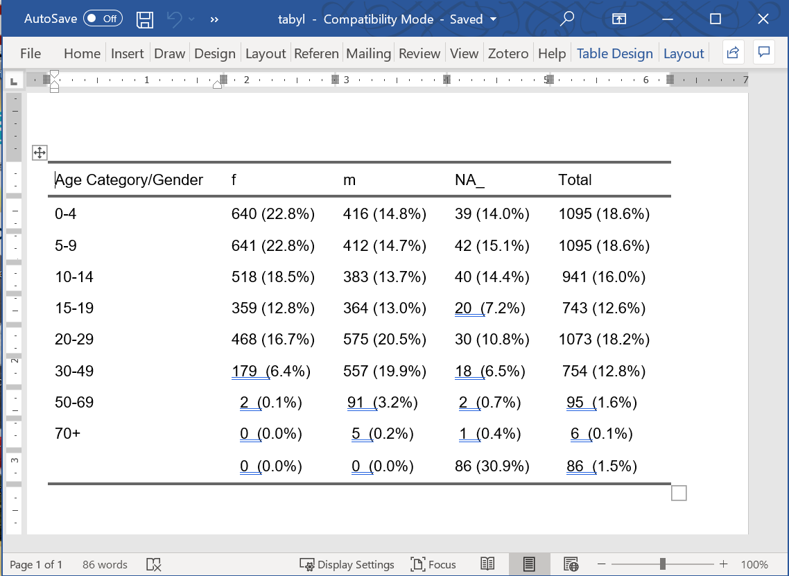

Statistics

You can apply statistical tests on tabyls, like chisq.test() or fisher.test() from the stats package, as shown below. Note missing values are not allowed so they are excluded from the tabyl with show_na = FALSE.

age_by_outcome <- linelist %>% 
  tabyl(age_cat, outcome, show_na = FALSE) 

chisq.test(age_by_outcome)


    Pearson's Chi-squared test

data:  age_by_outcome
X-squared = 6.4931, df = 7, p-value = 0.4835

dplyr package

dplyr is part of the tidyverse packages and is an very common data management tool. Creating tables with dplyr functions summarise() and count() is a useful approach to calculating summary statistics, summarize by group, or pass tables to ggplot().

summarise() creates a new, summary data frame. If the data are ungrouped, it will return a one-row dataframe with the specified summary statistics of the entire data frame. If the data are grouped, the new data frame will have one row per group.

Within the summarise() parentheses, you provide the names of each new summary column followed by an equals sign and a statistical function to apply.

Tip

The summarise function works with both UK and US spelling (summarise() and summarize()).

Get counts

The most simple function to apply within summarise() is n(). Leave the parentheses empty to count the number of rows.

linelist %>%                 # begin with linelist
  summarise(n_rows = n())    # return new summary dataframe with column n_rows

  n_rows
1   5888

This gets more interesting if we have grouped the data beforehand.

linelist %>% 
  group_by(age_cat) %>%     # group data by unique values in column age_cat
  summarise(n_rows = n())   # return number of rows *per group*

# A tibble: 9 × 2
  age_cat n_rows
  <fct>    <int>
1 0-4       1095
2 5-9       1095
3 10-14      941
4 15-19      743
5 20-29     1073
6 30-49      754
7 50-69       95
8 70+          6
9 <NA>        86

The above command can be shortened by using the count() function instead. count() does the following:

Groups the data by the columns provided to it
Summarises them with n() (creating column n)
Un-groups the data

linelist %>% 
  count(age_cat)

  age_cat    n
1     0-4 1095
2     5-9 1095
3   10-14  941
4   15-19  743
5   20-29 1073
6   30-49  754
7   50-69   95
8     70+    6
9    <NA>   86

You can change the name of the counts column from the default n to something else by specifying it to name =.

Tabulating counts of two or more grouping columns are still returned in “long” format, with the counts in the n column.

linelist %>% 
  count(age_cat, outcome)

   age_cat outcome   n
1      0-4   Death 471
2      0-4 Recover 364
3      0-4    <NA> 260
4      5-9   Death 476
5      5-9 Recover 391
6      5-9    <NA> 228
7    10-14   Death 438
8    10-14 Recover 303
9    10-14    <NA> 200
10   15-19   Death 323
11   15-19 Recover 251
12   15-19    <NA> 169
13   20-29   Death 477
14   20-29 Recover 367
15   20-29    <NA> 229
16   30-49   Death 329
17   30-49 Recover 238
18   30-49    <NA> 187
19   50-69   Death  33
20   50-69 Recover  38
21   50-69    <NA>  24
22     70+   Death   3
23     70+ Recover   3
24    <NA>   Death  32
25    <NA> Recover  28
26    <NA>    <NA>  26

Show all levels

If you are tabling a column of class factor you can ensure that all levels are shown (not just the levels with values in the data) by adding .drop = FALSE into the summarise() or count() command.

This technique is useful to standardise your tables/plots. For example if you are creating figures for multiple sub-groups, or repeatedly creating the figure for routine reports. In each of these circumstances, the presence of values in the data may fluctuate, but you can define levels that remain constant.

Proportions

Proportions can be added by piping the table to mutate() to create a new column. Define the new column as the counts column (n by default) divided by the sum() of the counts column (this will return a proportion).

Note that in this case, sum() in the mutate() command will return the sum of the whole column n for use as the proportion denominator. If sum() is used in grouped data (e.g. if the mutate() immediately followed a group_by() command), it will return sums by group. As stated just above, count() finishes its actions by ungrouping. Thus, in this scenario we get full column proportions.

To easily display percents, you can wrap the proportion in the function percent() from the package scales (note this convert to class character).

age_summary <- linelist %>% 
  count(age_cat) %>%                     # group and count by gender (produces "n" column)
  mutate(                                # create percent of column - note the denominator
    percent = scales::percent(n / sum(n))) 

# print
age_summary

  age_cat    n percent
1     0-4 1095  18.60%
2     5-9 1095  18.60%
3   10-14  941  15.98%
4   15-19  743  12.62%
5   20-29 1073  18.22%
6   30-49  754  12.81%
7   50-69   95   1.61%
8     70+    6   0.10%
9    <NA>   86   1.46%

Below is a method to calculate proportions within groups. It relies on different levels of data grouping being selectively applied and removed. First, the data are grouped on outcome via group_by(). Then, count() is applied. This function further groups the data by age_cat and returns counts for each outcome-age-cat combination. Importantly - as it finishes its process, count() also ungroups the age_cat grouping, so the only remaining data grouping is the original grouping by outcome. Thus, the final step of calculating proportions (denominator sum(n)) is still grouped by outcome.

age_by_outcome <- linelist %>%                  # begin with linelist
  group_by(outcome) %>%                         # group by outcome 
  count(age_cat) %>%                            # group and count by age_cat, and then remove age_cat grouping
  mutate(percent = scales::percent(n / sum(n))) # calculate percent - note the denominator is by outcome group

Plotting

To display a “long” table output like the above with ggplot() is relatively straight-forward. The data are naturally in “long” format, which is naturally accepted by ggplot().

linelist %>%                      # begin with linelist
  count(age_cat, outcome) %>%     # group and tabulate counts by two columns
  ggplot()+                       # pass new data frame to ggplot
    geom_col(                     # create bar plot
      mapping = aes(   
        x = outcome,              # map outcome to x-axis
        fill = age_cat,           # map age_cat to the fill
        y = n))                   # map the counts column `n` to the height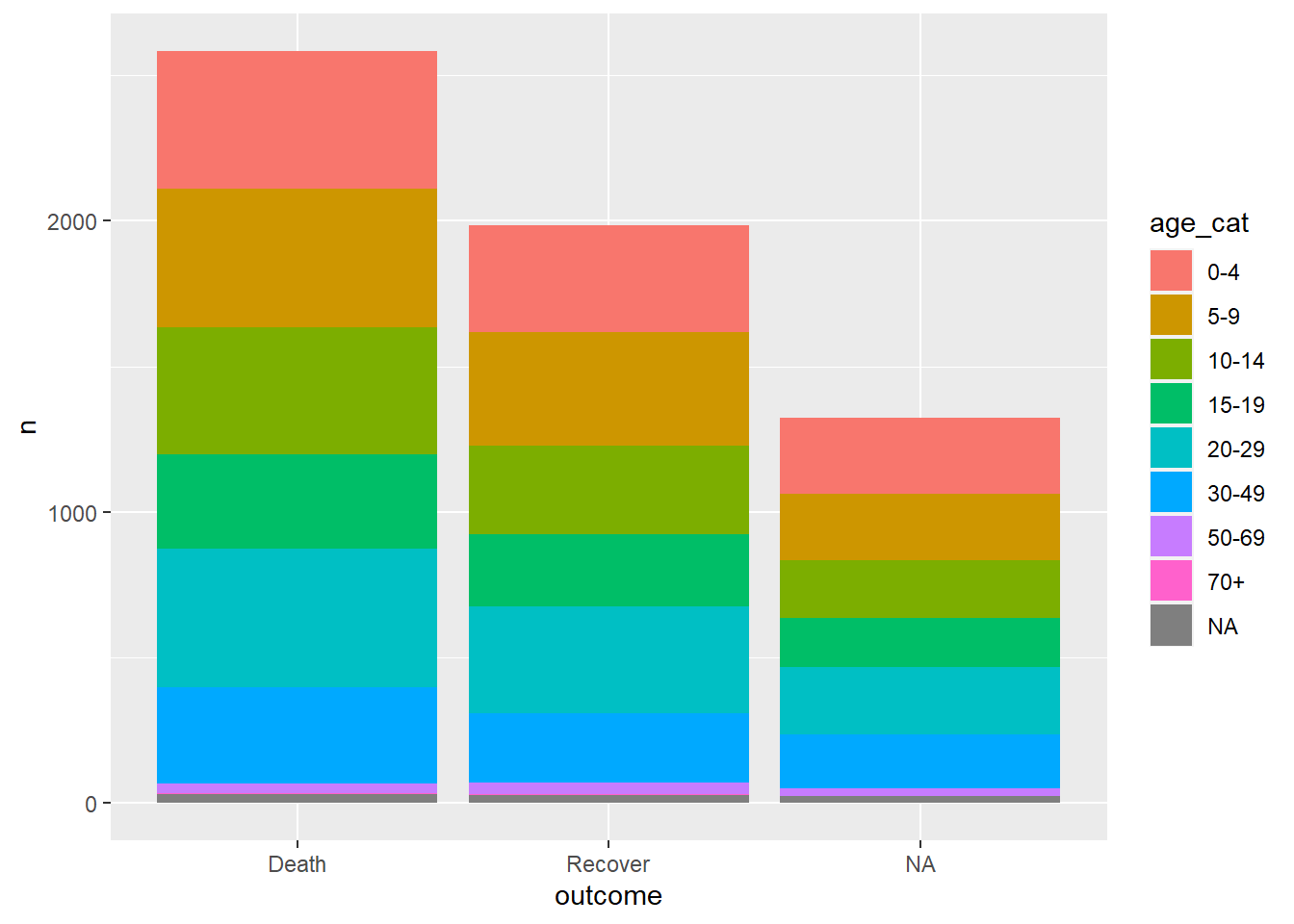

Summary statistics

One major advantage of dplyr and summarise() is the ability to return more advanced statistical summaries like median(), mean(), max(), min(), sd() (standard deviation), and percentiles. You can also use sum() to return the number of rows that meet certain logical criteria. As above, these outputs can be produced for the whole data frame set, or by group.

The syntax is the same - within the summarise() parentheses you provide the names of each new summary column followed by an equals sign and a statistical function to apply. Within the statistical function, give the column(s) to be operated on and any relevant arguments (e.g. na.rm = TRUE for most mathematical functions).

You can also use sum() to return the number of rows that meet a logical criteria. The expression within is counted if it evaluates to TRUE. For example:

sum(age_years < 18, na.rm=T)
sum(gender == "male", na.rm=T)
sum(response %in% c("Likely", "Very Likely"))

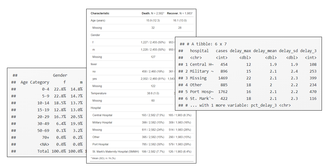
Below, linelist data are summarised to describe the days delay from symptom onset to hospital admission (column days_onset_hosp), by hospital.

summary_table <- linelist %>%                                        # begin with linelist, save out as new object
  group_by(hospital) %>%                                             # group all calculations by hospital
  summarise(                                                         # only the below summary columns will be returned
    cases       = n(),                                                # number of rows per group
    delay_max   = max(days_onset_hosp, na.rm = T),                    # max delay
    delay_mean  = round(mean(days_onset_hosp, na.rm=T), digits = 1),  # mean delay, rounded
    delay_sd    = round(sd(days_onset_hosp, na.rm = T), digits = 1),  # standard deviation of delays, rounded
    delay_3     = sum(days_onset_hosp >= 3, na.rm = T),               # number of rows with delay of 3 or more days
    pct_delay_3 = scales::percent(delay_3 / cases)                    # convert previously-defined delay column to percent 
  )

summary_table  # print

# A tibble: 6 × 7
  hospital               cases delay_max delay_mean delay_sd delay_3 pct_delay_3
  <chr>                  <int>     <dbl>      <dbl>    <dbl>   <int> <chr>      
1 Central Hospital         454        12        1.9      1.9     108 24%        
2 Military Hospital        896        15        2.1      2.4     253 28%        
3 Missing                 1469        22        2.1      2.3     399 27%        
4 Other                    885        18        2        2.2     234 26%        
5 Port Hospital           1762        16        2.1      2.2     470 27%        
6 St. Mark's Maternity …   422        18        2.1      2.3     116 27%

Some tips:

Use sum() with a logic statement to “count” rows that meet certain criteria (==)
Note the use of na.rm = TRUE within mathematical functions like sum(), otherwise NA will be returned if there are any missing values
Use the function percent() from the scales package to easily convert to percents
- Set accuracy = to 0.1 or 0.01 to ensure 1 or 2 decimal places respectively
Use round() from base R to specify decimals
To calculate these statistics on the entire dataset, use summarise() without group_by()
You may create columns for the purposes of later calculations (e.g. denominators) that you eventually drop from your data frame with select().

Conditional statistics

You may want to return conditional statistics - e.g. the maximum of rows that meet certain criteria. This can be done by subsetting the column with brackets [ ]. The example below returns the maximum temperature for patients classified having or not having fever. Be aware however - it may be more appropriate to add another column to the group_by() command and pivot_wider() (as demonstrated below).

linelist %>% 
  group_by(hospital) %>% 
  summarise(
    max_temp_fvr = max(temp[fever == "yes"], na.rm = T),
    max_temp_no = max(temp[fever == "no"], na.rm = T)
  )

# A tibble: 6 × 3
  hospital                             max_temp_fvr max_temp_no
  <chr>                                       <dbl>       <dbl>
1 Central Hospital                             40.4        38  
2 Military Hospital                            40.5        38  
3 Missing                                      40.6        38  
4 Other                                        40.8        37.9
5 Port Hospital                                40.6        38  
6 St. Mark's Maternity Hospital (SMMH)         40.6        37.9

Glueing together

The function str_glue() from stringr is useful to combine values from several columns into one new column. In this context this is typically used after the summarise() command.

Below, the summary_table data frame (created above) is mutated such that columns delay_mean and delay_sd are combined, parentheses formating is added to the new column, and their respective old columns are removed.

Then, to make the table more presentable, a total row is added with adorn_totals() from janitor (which ignores non-numeric columns). Lastly, we use select() from dplyr to both re-order and rename to nicer column names.
Now you could pass to flextable and print the table to Word, .png, .jpeg, .html, Powerpoint, RMarkdown, etc.! .

summary_table %>% 
  mutate(delay = str_glue("{delay_mean} ({delay_sd})")) %>%  # combine and format other values
  select(-c(delay_mean, delay_sd)) %>%                       # remove two old columns   
  adorn_totals(where = "row") %>%                            # add total row
  select(                                                    # order and rename cols
    "Hospital Name"   = hospital,
    "Cases"           = cases,
    "Max delay"       = delay_max,
    "Mean (sd)"       = delay,
    "Delay 3+ days"   = delay_3,
    "% delay 3+ days" = pct_delay_3
    )

                        Hospital Name Cases Max delay Mean (sd) Delay 3+ days
                     Central Hospital   454        12 1.9 (1.9)           108
                    Military Hospital   896        15 2.1 (2.4)           253
                              Missing  1469        22 2.1 (2.3)           399
                                Other   885        18   2 (2.2)           234
                        Port Hospital  1762        16 2.1 (2.2)           470
 St. Mark's Maternity Hospital (SMMH)   422        18 2.1 (2.3)           116
                                Total  5888       101         -          1580
 % delay 3+ days
             24%
             28%
             27%
             26%
             27%
             27%
               -

Percentiles

Percentiles and quantiles in dplyr deserve a special mention. To return quantiles, use quantile() with the defaults or specify the value(s) you would like with probs =.

# get default percentile values of age (0%, 25%, 50%, 75%, 100%)
linelist %>% 
  summarise(age_percentiles = quantile(age_years, na.rm = TRUE))

Warning: Returning more (or less) than 1 row per `summarise()` group was deprecated in
dplyr 1.1.0.
ℹ Please use `reframe()` instead.
ℹ When switching from `summarise()` to `reframe()`, remember that `reframe()`
  always returns an ungrouped data frame and adjust accordingly.

  age_percentiles
1               0
2               6
3              13
4              23
5              84

# get manually-specified percentile values of age (5%, 50%, 75%, 98%)
linelist %>% 
  summarise(
    age_percentiles = quantile(
      age_years,
      probs = c(.05, 0.5, 0.75, 0.98), 
      na.rm=TRUE)
    )

Warning: Returning more (or less) than 1 row per `summarise()` group was deprecated in
dplyr 1.1.0.
ℹ Please use `reframe()` instead.
ℹ When switching from `summarise()` to `reframe()`, remember that `reframe()`
  always returns an ungrouped data frame and adjust accordingly.

  age_percentiles
1               1
2              13
3              23
4              48

If you want to return quantiles by group, you may encounter long and less useful outputs if you simply add another column to group_by(). So, try this approach instead - create a column for each quantile level desired.

# get manually-specified percentile values of age (5%, 50%, 75%, 98%)
linelist %>% 
  group_by(hospital) %>% 
  summarise(
    p05 = quantile(age_years, probs = 0.05, na.rm=T),
    p50 = quantile(age_years, probs = 0.5, na.rm=T),
    p75 = quantile(age_years, probs = 0.75, na.rm=T),
    p98 = quantile(age_years, probs = 0.98, na.rm=T)
    )

# A tibble: 6 × 5
  hospital                               p05   p50   p75   p98
  <chr>                                <dbl> <dbl> <dbl> <dbl>
1 Central Hospital                         1    12    21  48  
2 Military Hospital                        1    13    24  45  
3 Missing                                  1    13    23  48.2
4 Other                                    1    13    23  50  
5 Port Hospital                            1    14    24  49  
6 St. Mark's Maternity Hospital (SMMH)     2    12    22  50.2

Summarise aggregated data

If you begin with aggregated data, using n() return the number of rows, not the sum of the aggregated counts. To get sums, use sum() on the data’s counts column.

For example, let’s say you are beginning with the data frame of counts below, called linelist_agg - it shows in “long” format the case counts by outcome and gender.

Below we create this example data frame of linelist case counts by outcome and gender (missing values removed for clarity).

linelist_agg <- linelist %>% 
  drop_na(gender, outcome) %>% 
  count(outcome, gender)

linelist_agg

  outcome gender    n
1   Death      f 1227
2   Death      m 1228
3 Recover      f  953
4 Recover      m  950

To sum the counts (in column n) by group you can use summarise() but set the new column equal to sum(n, na.rm=T). To add a conditional element to the sum operation, you can use the subset bracket [ ] syntax on the counts column.

linelist_agg %>% 
  group_by(outcome) %>% 
  summarise(
    total_cases  = sum(n, na.rm=T),
    male_cases   = sum(n[gender == "m"], na.rm=T),
    female_cases = sum(n[gender == "f"], na.rm=T))

# A tibble: 2 × 4
  outcome total_cases male_cases female_cases
  <chr>         <int>      <int>        <int>
1 Death          2455       1228         1227
2 Recover        1903        950          953

`across()` multiple columns

You can use summarise() across multiple columns using across(). This makes life easier when you want to calculate the same statistics for many columns. Place across() within summarise() and specify the following:

.cols = as either a vector of column names c() or “tidyselect” helper functions (explained below)
.fns = the function to perform (no parentheses) - you can provide multiple within a list()

Below, mean() is applied to several numeric columns. A vector of columns are named explicitly to .cols = and a single function mean is specified (no parentheses) to .fns =. Any additional arguments for the function (e.g. na.rm=TRUE) are provided after .fns =, separated by a comma.

It can be difficult to get the order of parentheses and commas correct when using across(). Remember that within across() you must include the columns, the functions, and any extra arguments needed for the functions.

linelist %>% 
  group_by(outcome) %>% 
  summarise(across(.cols = c(age_years, temp, wt_kg, ht_cm),  # columns
                   .fns = mean,                               # function
                   na.rm=T))                                  # extra arguments

Warning: There was 1 warning in `summarise()`.
ℹ In argument: `across(...)`.
ℹ In group 1: `outcome = "Death"`.
Caused by warning:
! The `...` argument of `across()` is deprecated as of dplyr 1.1.0.
Supply arguments directly to `.fns` through an anonymous function instead.

  # Previously
  across(a:b, mean, na.rm = TRUE)

  # Now
  across(a:b, \(x) mean(x, na.rm = TRUE))

# A tibble: 3 × 5
  outcome age_years  temp wt_kg ht_cm
  <chr>       <dbl> <dbl> <dbl> <dbl>
1 Death        15.9  38.6  52.6  125.
2 Recover      16.1  38.6  52.5  125.
3 <NA>         16.2  38.6  53.0  125.

Multiple functions can be run at once. Below the functions mean and sd are provided to .fns = within a list(). You have the opportunity to provide character names (e.g. “mean” and “sd”) which are appended in the new column names.

linelist %>% 
  group_by(outcome) %>% 
  summarise(across(.cols = c(age_years, temp, wt_kg, ht_cm), # columns
                   .fns = list("mean" = mean, "sd" = sd),    # multiple functions 
                   na.rm=T))                                 # extra arguments

# A tibble: 3 × 9
  outcome age_years_mean age_years_sd temp_mean temp_sd wt_kg_mean wt_kg_sd
  <chr>            <dbl>        <dbl>     <dbl>   <dbl>      <dbl>    <dbl>
1 Death             15.9         12.3      38.6   0.962       52.6     18.4
2 Recover           16.1         13.0      38.6   0.997       52.5     18.6
3 <NA>              16.2         12.8      38.6   0.976       53.0     18.9
# ℹ 2 more variables: ht_cm_mean <dbl>, ht_cm_sd <dbl>

Here are those “tidyselect” helper functions you can provide to .cols = to select columns:

everything() - all other columns not mentioned
last_col() - the last column
where() - applies a function to all columns and selects those which are TRUE
starts_with() - matches to a specified prefix. Example: starts_with("date")
ends_with() - matches to a specified suffix. Example: ends_with("_end")
contains() - columns containing a character string. Example: contains("time")
matches() - to apply a regular expression (regex). Example: contains("[pt]al")
num_range() -
any_of() - matches if column is named. Useful if the name might not exist. Example: any_of(date_onset, date_death, cardiac_arrest)

For example, to return the mean of every numeric column use where() and provide the function as.numeric() (without parentheses). All this remains within the across() command.

linelist %>% 
  group_by(outcome) %>% 
  summarise(across(
    .cols = where(is.numeric),  # all numeric columns in the data frame
    .fns = mean,
    na.rm=T))

# A tibble: 3 × 12
  outcome generation   age age_years   lon   lat wt_kg ht_cm ct_blood  temp
  <chr>        <dbl> <dbl>     <dbl> <dbl> <dbl> <dbl> <dbl>    <dbl> <dbl>
1 Death         16.7  15.9      15.9 -13.2  8.47  52.6  125.     21.3  38.6
2 Recover       16.4  16.2      16.1 -13.2  8.47  52.5  125.     21.1  38.6
3 <NA>          16.5  16.3      16.2 -13.2  8.47  53.0  125.     21.2  38.6
# ℹ 2 more variables: bmi <dbl>, days_onset_hosp <dbl>

Total rows

When summarise() operates on grouped data it does not automatically produce “total” statistics. Below, two approaches to adding a total row are presented:

janitor’s `adorn_totals()`

If your table consists only of counts or proportions/percents that can be summed into a total, then you can add sum totals using janitor’s adorn_totals() as described in the section above. Note that this function can only sum the numeric columns - if you want to calculate other total summary statistics see the next approach with dplyr.

Below, linelist is grouped by gender and summarised into a table that described the number of cases with known outcome, deaths, and recovered. Piping the table to adorn_totals() adds a total row at the bottom reflecting the sum of each column. The further adorn_*() functions adjust the display as noted in the code.

linelist %>% 
  group_by(gender) %>%
  summarise(
    known_outcome = sum(!is.na(outcome)),           # Number of rows in group where outcome is not missing
    n_death  = sum(outcome == "Death", na.rm=T),    # Number of rows in group where outcome is Death
    n_recover = sum(outcome == "Recover", na.rm=T), # Number of rows in group where outcome is Recovered
  ) %>% 
  adorn_totals() %>%                                # Adorn total row (sums of each numeric column)
  adorn_percentages("col") %>%                      # Get column proportions
  adorn_pct_formatting() %>%                        # Convert proportions to percents
  adorn_ns(position = "front")                      # display % and counts (with counts in front)

 gender  known_outcome        n_death      n_recover
      f 2,180  (47.8%) 1,227  (47.5%)   953  (48.1%)
      m 2,178  (47.7%) 1,228  (47.6%)   950  (47.9%)
   <NA>   207   (4.5%)   127   (4.9%)    80   (4.0%)
  Total 4,565 (100.0%) 2,582 (100.0%) 1,983 (100.0%)

`summarise()` on “total” data and then `bind_rows()`

If your table consists of summary statistics such as median(), mean(), etc, the adorn_totals() approach shown above will not be sufficient. Instead, to get summary statistics for the entire dataset you must calculate them with a separate summarise() command and then bind the results to the original grouped summary table. You can make a summary table of outcome by hospital with group_by() and summarise() like this:

by_hospital <- linelist %>% 
  filter(!is.na(outcome) & hospital != "Missing") %>%  # Remove cases with missing outcome or hospital
  group_by(hospital, outcome) %>%                      # Group data
  summarise(                                           # Create new summary columns of indicators of interest
    N = n(),                                            # Number of rows per hospital-outcome group     
    ct_value = median(ct_blood, na.rm=T))               # median CT value per group
  
by_hospital # print table

# A tibble: 10 × 4
# Groups:   hospital [5]
   hospital                             outcome     N ct_value
   <chr>                                <chr>   <int>    <dbl>
 1 Central Hospital                     Death     193       22
 2 Central Hospital                     Recover   165       22
 3 Military Hospital                    Death     399       21
 4 Military Hospital                    Recover   309       22
 5 Other                                Death     395       22
 6 Other                                Recover   290       21
 7 Port Hospital                        Death     785       22
 8 Port Hospital                        Recover   579       21
 9 St. Mark's Maternity Hospital (SMMH) Death     199       22
10 St. Mark's Maternity Hospital (SMMH) Recover   126       22

To get the totals, run the same summarise() command but only group the data by outcome (not by hospital), like this:

totals <- linelist %>% 
      filter(!is.na(outcome) & hospital != "Missing") %>%
      group_by(outcome) %>%                            # Grouped only by outcome, not by hospital    
      summarise(
        N = n(),                                       # These statistics are now by outcome only     
        ct_value = median(ct_blood, na.rm=T))

totals # print table

# A tibble: 2 × 3
  outcome     N ct_value
  <chr>   <int>    <dbl>
1 Death    1971       22
2 Recover  1469       22

We can bind these two data frames together. Note that by_hospital has 4 columns whereas totals has 3 columns. By using bind_rows(), the columns are combined by name, and any extra space is filled in with NA (e.g the column hospital values for the two new totals rows). After binding the rows, we convert these empty spaces to “Total” using replace_na().

table_long <- bind_rows(by_hospital, totals) %>% 
  mutate(hospital = replace_na(hospital, "Total"))

Here is the new table with “Total” rows at the bottom.

This table is in a “long” format, which may be what you want. Optionally, you can pivot this table wider to make it more readable (which we will learn about later). You can also add more columns, and arrange it nicely. This code is below.

table_long %>% 
  
  # Pivot wider and format
  ########################
  mutate(hospital = replace_na(hospital, "Total")) %>% 
  pivot_wider(                                         # Pivot from long to wide
    values_from = c(ct_value, N),                       # new values are from ct and count columns
    names_from = outcome) %>%                           # new column names are from outcomes
  mutate(                                              # Add new columns
    N_Known = N_Death + N_Recover,                               # number with known outcome
    Pct_Death = scales::percent(N_Death / N_Known, 0.1),         # percent cases who died (to 1 decimal)
    Pct_Recover = scales::percent(N_Recover / N_Known, 0.1)) %>% # percent who recovered (to 1 decimal)
  select(                                              # Re-order columns
    hospital, N_Known,                                   # Intro columns
    N_Recover, Pct_Recover, ct_value_Recover,            # Recovered columns
    N_Death, Pct_Death, ct_value_Death)  %>%             # Death columns
  arrange(N_Known)                                  # Arrange rows from lowest to highest (Total row at bottom)

# A tibble: 6 × 8
# Groups:   hospital [6]
  hospital      N_Known N_Recover Pct_Recover ct_value_Recover N_Death Pct_Death
  <chr>           <int>     <int> <chr>                  <dbl>   <int> <chr>    
1 St. Mark's M…     325       126 38.8%                     22     199 61.2%    
2 Central Hosp…     358       165 46.1%                     22     193 53.9%    
3 Other             685       290 42.3%                     21     395 57.7%    
4 Military Hos…     708       309 43.6%                     22     399 56.4%    
5 Port Hospital    1364       579 42.4%                     21     785 57.6%    
6 Total            3440      1469 42.7%                     22    1971 57.3%    
# ℹ 1 more variable: ct_value_Death <dbl>

In the next chapter we’ll see how to create an attractive visualization of the table, as shown here:

Hospital	Total cases with known outcome	Recovered			Died
Hospital	Total cases with known outcome	Total	% of cases	Median CT values	Total	% of cases	Median CT values
St. Mark's Maternity Hospital (SMMH)	325	126	38.8%	22	199	61.2%	22
Central Hospital	358	165	46.1%	22	193	53.9%	22
Other	685	290	42.3%	21	395	57.7%	22
Military Hospital	708	309	43.6%	22	399	56.4%	21
Missing	1,125	514	45.7%	21	611	54.3%	21
Port Hospital	1,364	579	42.4%	21	785	57.6%	22
Total	3,440	1,469	42.7%	22	1,971	57.3%	22

base R

You can use the function table() to tabulate and cross-tabulate columns. Unlike the options above, you must specify the dataframe each time you reference a column name, as shown below.

Warning

NA (missing) values will not be tabulated unless you include the argument useNA = "always" (which could also be set to “no” or “ifany”).

Tip

You can use the %$% from magrittr to remove the need for repeating data frame calls within base functions. For example the below could be written linelist %$% table(outcome, useNA = "always")

table(linelist$outcome, useNA = "always")


  Death Recover    <NA> 
   2582    1983    1323

Multiple columns can be cross-tabulated by listing them one after the other, separated by commas. Optionally, you can assign each column a “name” like Outcome = linelist$outcome.

age_by_outcome <- table(linelist$age_cat, linelist$outcome, useNA = "always") # save table as object
age_by_outcome   # print table

       
        Death Recover <NA>
  0-4     471     364  260
  5-9     476     391  228
  10-14   438     303  200
  15-19   323     251  169
  20-29   477     367  229
  30-49   329     238  187
  50-69    33      38   24
  70+       3       3    0
  <NA>     32      28   26

Proportions

To return proportions, passing the above table to the function prop.table(). Use the margins = argument to specify whether you want the proportions to be of rows (1), of columns (2), or of the whole table (3). For clarity, we pipe the table to the round() function from base R, specifying 2 digits.

# get proportions of table defined above, by rows, rounded
prop.table(age_by_outcome, 1) %>% round(2)

       
        Death Recover <NA>
  0-4    0.43    0.33 0.24
  5-9    0.43    0.36 0.21
  10-14  0.47    0.32 0.21
  15-19  0.43    0.34 0.23
  20-29  0.44    0.34 0.21
  30-49  0.44    0.32 0.25
  50-69  0.35    0.40 0.25
  70+    0.50    0.50 0.00
  <NA>   0.37    0.33 0.30

Totals

To add row and column totals, pass the table to addmargins(). This works for both counts and proportions.

addmargins(age_by_outcome)

       
        Death Recover <NA>  Sum
  0-4     471     364  260 1095
  5-9     476     391  228 1095
  10-14   438     303  200  941
  15-19   323     251  169  743
  20-29   477     367  229 1073
  30-49   329     238  187  754
  50-69    33      38   24   95
  70+       3       3    0    6
  <NA>     32      28   26   86
  Sum    2582    1983 1323 5888

Descriptive analysis

Load packages

Import data

Browse data

Summary statistics

janitor package

Simple tabyl

Cross-tabulation

“Adorning” the tabyl

Printing the tabyl

Use on other tables

Saving the tabyl

Statistics

dplyr package

Get counts

Show all levels

Proportions

Plotting

Summary statistics

Conditional statistics

Glueing together

Percentiles

Summarise aggregated data

across() multiple columns

Total rows

janitor’s adorn_totals()

summarise() on “total” data and then bind_rows()

base R

Proportions

Totals

`across()` multiple columns

janitor’s `adorn_totals()`

`summarise()` on “total” data and then `bind_rows()`